[Review] SDE

앞서 Review한 Diffusion Model과, score-based model을 모두 통합하는 generalized framework를 제시한, Score-Based Generative Modeling through Stochastic Differential Equations (SDE) 논문을 살펴보자. 이것도 Yang Song 씨의 논문이다.

1. Introduction

Training data에 점차 증가하는 noise를 주입하면서 corrupting한 뒤, reverse process를 통해 이 corrupting process를 학습하는 생성 모델은 2가지가 있다.

SMLD

[My NCSN Review]

여기서 SMLD는 Denoising Score Matching with Langevin Dynamics의 줄임말로, NCSN이랑 동일한 것이다. $\sigma_{i}$가 $\frac{\sigma_{1}}{\sigma_{2}}=…=\frac{\sigma_{L-1}}{\sigma_{N}}<1$를 만족하는 noise들이라고 하자. 그리고 \(p_{\sigma}(\widetilde{x} \mid x):=N(\widetilde{x} ; x, \sigma^{2}I)\)일 때 \(p_{\sigma}(x):=\int p_{data}(t)p_{\sigma}(x \mid t)dt\)로 주어지는 perturbed data distribution를 고려하자. 이 때, NCSN에서 다루었듯이 충분히 작은 noise level인 $\sigma_{1}:=\sigma_{min}$에 대해서는 $p_{\sigma_{min}}(x)\sim p_{data}(x)$ 이면서도 충분히 큰 noise level인 $\sigma_{N}:=\sigma_{max}$에 대해서는 $p_{\sigma_{max}}(x)\sim N(0,\sigma_{max}^{2}I)$를 만족한다. 그랬을 때 NCSN model은 denoising score matching의 weighted sum으로 하나의 score-based model을 학습한다. 즉,

\[\theta^{*}:=\underset{\theta}{arg\,min\,}\sum_{i=1}^{N} \sigma_{i}^{2}\mathbb{E}_{p_{data}}\mathbb{E}_{p_{\sigma_{i}}(\widetilde{x} \mid x)}[\|s_{\theta}(\widetilde{x},\sigma_{i})-\nabla_{\widetilde{x}}log\,p_{\sigma_{i}}(\widetilde{x} \mid x)\|_{2}^2] \; \\ where\;\; \nabla_{\widetilde{x}}log\,p_{\sigma_{i}}(\widetilde{x} \mid x)=-\frac{\widetilde{x}-x}{\sigma_{i}^{2}}\;, p_{\sigma_{i}}(\widetilde{x} \mid x)\sim N(x,\sigma_{i}^{2}I)\]

그리고 Inference 시에는 M-step annealed Langevin MCMC를 통해 각 noise level에서 sample을 얻는다.

\[\widetilde{x}_{i}^{m}=\widetilde{x}_{i-1}^{m}+\frac{\epsilon_{i}}{2}s_{\theta^{*}}(\widetilde{x}_{i-1}^{m},\sigma_{i})+\sqrt{\epsilon_{i}}z_{i}^{m} \\ where\;z_{i}^{m}\sim N(0,I), m=1,2,...,M, i=N,N-1,...,1 \\ x_{N}^{0}\sim N(x\mid 0,\sigma_{max}^{2}I),\; x_{i}^{0}=x_{i+1}^{M}\;\forall i<N\]

DDPM

[My DDPM Review]

$\beta_{t}:10^{-4}\searrow 0.02$인 noise level에 대해서, training data $x_{0}\sim p_{data}(x)$에 대해 discrete Markov chain ${x_{0},…,x_{N}}$을 다음과 같이 구성한다: \(p(x_{i}\mid x_{i-1})=N(x_{i};\sqrt{1-\beta _{i}}X_{i-1}, \beta _{i}I)\). 한 방에 적으면, \(p_{\alpha_{i}}(x_{i}\mid x_{0})=N(x_{i};\sqrt{\alpha_{i}}x_{0},(1-\alpha_{i})I)\;where\;\alpha_{i}=\prod_{j=1}^{i}(1-\beta_{j})\). 마찬가지로 \(p_{\alpha_{i}}(x):=\int p_{data}(t)p_{\alpha_{i}}(x \mid t)dt\) 로 주어지는 perturbed data distribution를 고려할 때, reverse process distribution을 parametrize한 \(p_{\theta}(x_{i-1}\mid x_{i})=N(x_{i-1};\frac{1}{\sqrt{1-\beta_{i}}}(x_{i}+\beta_{i}s_{\theta}(x_{i},i)),\beta_{i}I)\)를 학습한다. 이 때, \(s_{\theta}(x_{i},i)\)는 noisy input 분포 \(p_{\alpha_{i}}(x)\)의 score와 matching하여 학습한다. 즉,

\[\theta^{*}:=\underset{\theta}{arg\,min\,}\sum_{i=1}^{N} (1-\alpha_{i})\mathbb{E}_{p_{data}}\mathbb{E}_{p_{\alpha_{i}}(\widetilde{x} \mid x)}[\|s_{\theta}(\widetilde{x},i)-\nabla_{\widetilde{x}}log\,p_{\alpha_{i}}(\widetilde{x} \mid x)\|_{2}^2] \; \\ where\;\; p_{\alpha_{i}}(\widetilde{x} \mid x)\sim N(\sqrt{\alpha_{i}}x,(1-\alpha_{i})I)\]

그리고 inference 시에는 reverse Markov chain을 따라 Gaussian noise로부터 sample을 얻는다.

\[x_{i-1}=\frac{1}{\sqrt{1-\beta_{i}}}(x_{i}+\beta_{i}s_{\theta^{*}}(x_{i},i))+\sqrt{\beta_{i}}z_{i} \\ where\;\; x_{N},z_{i}\sim N(0,I)\,\forall i,\;i=N,N-1,...,1\]

참고로 논문에서 저자는 이 sampling 방법을 ancestral sampling이라고 부르고 있다.

참고해야 될 부분은 두 모델 모두 optimal model $s_{\theta^{*}}(x_{i},i)$를 perturbed data distribution의 score(gradient of log-likelihood)와 matching 하고 있으며, 여러 noise level에 대한 score matching 간의 weighted sum으로 학습하고 있다. 이 때, coefficient는 NCSN에서는 $\sigma_{i}^{2}$, DDPM에서는 $1-\alpha_{i}$인데 두 상수 모두 각각의 noise level $i$에 대해서 $\frac{1}{E[|\nabla_{\widetilde{x}}log\,p_{i}(\widetilde{x} \mid x)|_{2}^2]}$에 비례하도록 하여 weight를 통해 score matching term간 noise level에 따른 차이가 없도록 하였다. (NCSN은 실험적으로 결정한 것이고, DDPM은 수식에 따라 결정된 것이다.)

위에 있는 수식이 DDPM 논문에 있는 수식이랑 겉으로 보기에는 다른 것 처럼 보이지만, 사실 SMLD와 동일한 형태(score-matching 형태)로 보일 수 있도록 저자가 편의를 위해 바꾼 것이다. 살펴보자면, DDPM의 forward distribution \(p_{\alpha_{i}}(x_{i}\mid x_{0})=N(x_{i};\sqrt{\alpha_{i}}x_{0},(1-\alpha_{i})I)\)를 우리는 Reparameterization trick을 이용하여, 다시 말해 Gaussian 분포에서 얻은 sample \(\epsilon\)을 variance에 곱한걸 평균에 더해서 \(x_{i}\)를 얻었었다: \(x_{i}=\sqrt{\alpha_{i}}x_{0}+\sqrt{1-\alpha_{i}}\epsilon_{i}\;where\;\epsilon_{i}\sim N(0,I)\). 그랬을 때, 위 식에서 \(\nabla_{\widetilde{x}}log\,p_{\alpha_{i}}(\widetilde{x} \mid x)=-\,\frac{\widetilde{x}-\sqrt{\alpha_{i}}x_{0}}{1-\alpha_{i}}=-\,\frac{\epsilon_{i}}{\sqrt{1-\alpha_{i}}}\)가 되는 걸 알 수 있다. 기존에 DDPM에서 서술했던 방식의 Loss term은 \(\mathbb{E}_{N, x_{0}, \epsilon}[\|\epsilon_{\theta}(\widetilde{x},i)-\epsilon\|_{2}^2]\)로, noise를 학습하는 network라고 봤지만 사실 \(s_{\theta}(\widetilde{x},i):=-\,\frac{\epsilon_{\theta}(\widetilde{x},i)}{\sqrt{1-\alpha_{i}}}\)로 본다면 \(\alpha_{i}\)는 상수이기 때문에 \(\epsilon_{\theta}(\widetilde{x},i)\)를 학습하는 것과 \(s_{\theta}(\widetilde{x},i)\)를 학습하는 건 똑같은 말이 된다. 따라서, \(\sum_{i=1}^{N} (1-\alpha_{i})\mathbb{E}_{p_{data}}\mathbb{E}_{p_{\alpha_{i}}(\widetilde{x} \mid x)}[\|s_{\theta}(\widetilde{x},i)-\nabla_{\widetilde{x}}log\,p_{\alpha_{i}}(\widetilde{x} \mid x)\|_{2}^2]=\mathbb{E}_{N, x_{0}, \epsilon}[\|\epsilon_{\theta}(\widetilde{x},i)-\epsilon\|_{2}^2]\) 임을 알 수 있다.

SDE

[SDE란]

SDE는 Stochastic process의 Differential Equation으로, \(dX(t)=f(t,X(t))dt+g(t,X(t))dW(t)\;,X(0)=X_{0}\)의 형태이다. 혹은, \(X(T)=X_{0}+\int_{0}^{T}f(s,X(s))dx + \int_{0}^{T}g(x,X(s))dW(s)\)의 형태이다. 이 때 두 번째 적분 term은 integrand/integrator 모두 Stochastic process인 Itô integral인데, 정확히는 모르겠지만 Riemann-Stieltjes 적분이랑 비슷하게 정의된다고 한다. (확실한 건 \(\int_{0}^{T}GdW(s)=\int_{0}^{T}GW'ds\)는 Brownian motion \(W(t)\)가 미분 불가능하므로, 이렇게 단순하게 풀리는 적분은 아니다.) 적분식으로 나타낸 이유는, SDE의 해를 위와 같은 적분 형태로 수치적으로 구하는 SDE integrator가 Euler-Maruyama, Runge-Kutta, Leimkuhler-Matthews 등 다양한 방법이 이미 알려져있기 때문이다. 그리고 위와 같은 SDE가, drift term f와 diffusion term g가 globally Lipscitz하면 unique strong solution을 가진다고 알려져있다.

또한, network의 forward pass나 backpropagation을 ODE/SDE Solver를 이용하는 ODE-Net과 같은 방식이 제안되었었다. [My ODE-Net Review]

2. Score-Based Generative Modeling with SDEs

“Score Matching”=”Solving SDE”를 아주 잘 나타내는 Toy Example이다.

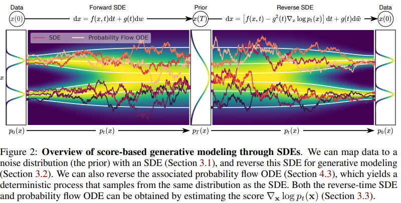
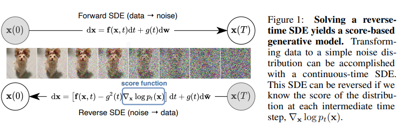
Forward SDE

우선 저자가 SDE를 떠올리게 된 이유는, DDPM에서의 discrete Markov chain을 contiuous Markov chain으로 일반화해보는 시도에서 이런 아이디어가 나왔을 것이라 생각된다. DDPM에서의 discrete time variable $i$가 아닌, continuous time variable $t\in [0,T]$를 고려한 diffusion process $\mathbf{x}(t)$를 고려한다. 이 때 $\mathbf{x}(0)$는 실제 데이터 분포 $p_{0}$의 i.i.d. sample이고, $\mathbf{x}(T)\sim p_{T}$, $p_{T}$는 Gaussian distribution와 같은 prior distribution이다.

그래서 이 diffusion process는 위에서 말한 Itô SDE의 solution으로 모델링할 수 있다. \(d\mathbf{x}=\mathbf{f}(\mathbf{x},t)dt+g(t)d\mathbf{w}\) 논문에서 활용한 SDE인데, diffusion coefficient를 stochastic process에 independent하고 matrix가 아닌 scalar function으로 가정하고 있다. \(\mathbf{x}(t)\)의 pdf를 \(p_{t}(\mathbf{x})\)라 하고, \(s<t\)일 때 \(\mathbf{x}(s)\)에서 \(\mathbf{x}(t)\)로의 transition kernel을 \(p_{st}(\mathbf{x}(t)\mid \mathbf{x}(s))\)로 한다.

Reverse SDE

prior distribution $p_{T}$로 부터 얻은 sample들 $\mathbf{x}(T)$로 부터 실제 데이터 분포에서의 sample $\mathbf{x}(0)$를 생성해낼 수 있는데, 위 diffusion process의 reverse 또한 마찬가지로 diffusion process이며 다음과 같은 SDE로 표현된다고 한다. [(Anderson, 1982)-Section 5 참고]

\[d\mathbf{x}=[\mathbf{f}(\mathbf{x},t)-g(t)^{2}\nabla_{\mathbf{x}}log\;p_{t}(\mathbf{x})]dt+g(t)d\overline{\mathbf{w}}\]

이 때, dt는 T에서 0으로 감소하는 negative timestep이고, \(\overline{\mathbf{w}}\)는 Wiener process이지만 time이 T에서 0으로 감소하는 방향. diffusion term은 forward SDE에서의 diffusion term과 동일한데, drift term은 forward SDE에서의 drift term에 score term을 추가해 dt의 궤도를 바꾸어주고 있다. 따라서, forward SDE의 solution \(p_{t}(\mathbf{x})\)의 score를 알면 sampling을 할 수 있게 된다.

그래서 NCSN이나 DDPM과 동일하게 score-matching을 기반으로 분포를 학습한다.

\[\theta^{*}:=\underset{\theta}{arg\,min\,}\mathbb{E}_{t}\Big\{\lambda(t) \mathbb{E}_{\mathbf{x}(0)}E_{\mathbf{x}(t) \mid \mathbf{x}(0)}[\|s_{\theta}(\mathbf{x}(t),t)-\nabla_{\mathbf{x}(t)}log\,p_{0t}(\mathbf{x}(t) \mid \mathbf{x}(0))\|_{2}^2]\Big\} \\ where\;\; \lambda:[0,T]\rightarrow \mathbb{R}_{>0}, t\sim Unif[0,T], \mathbf{x}(0)\sim p_{0}(\mathbf{x}), \mathbf{x}(t)\sim p_{0t}(\mathbf{x}(t)\mid \mathbf{x}(0))\]

여기서 \(\lambda(t)\)는 weight function으로, 마찬가지로 NCSN과 DDPM과 똑같이 \(\lambda(t)\propto \frac{1}{\mathbb{E}[\|\nabla_{\mathbf{x}(t)}log\,p_{0t}(\mathbf{x}(t) \mid \mathbf{x}(0))\|_{2}^2]}\)를 만족하도록 설정한다. 그리고 논문에서 위 score matching은 denoising score matching 방식이지만, sliced score matching와 같은 다른 방식도 적용할 수 있다고 말하고 있다.

결국 저 transition kernel \(p_{0t}(\mathbf{x}(t)\mid \mathbf{x}(0))\)를 알아야 되는데, drift coefficient \(\mathbf{f}(\mathbf{x},t)\)가 affine일 때 transition kernel은 항상 Gaussian distribution이고 평균과 분산에 대한 식이 explicit하게 알려져있다고 한다. [Section 5.5, Equation (5.50, 5.51) 참고] 만약 affine 하지 않다면 Kolmogorov’s forward equation을 풀거나 라는데 이건 잘 모르겠고 denoising score matching이 아닌 sliced score matching 방식을 채택해서 해당 transition kernel의 score를 구하지 않고, pytorch의 자동 도움을 얻는 방법으로 우회할 수 있다.

Appendix A. General Cases

Appendix A에서 \(d\mathbf{x}=\mathbf{f}(\mathbf{x},t)dt+g(t)d\mathbf{w}\) 로 주어진 SDE에서, diffusion coefficient가 일반적인 matrix \(\mathbf{G}(\mathbf{x},t)\)일 때에도 문제 없이 적용된다고 말하고 있다. Forward SDE가 \(d\mathbf{x}=\mathbf{f}(\mathbf{x},t)dt+\mathbf{G}(\mathbf{x},t)d\mathbf{w}\)로 주어졌을 때, Anderson 씨 [(Anderson, 1982)-Section 5 참고]에 의하면 reverse SDE는 다음과 같이 주어진다고 한다.

\[d\mathbf{x}=\{\mathbf{f}(\mathbf{x},t)-\nabla_{\mathbf{x}} \cdot [\mathbf{G}(\mathbf{x},t)\mathbf{G}(\mathbf{x},t)^{T}]-\mathbf{G}(\mathbf{x},t)\mathbf{G}(\mathbf{x},t)^{T} \nabla_{\mathbf{x}}log\;p_{t}(\mathbf{x})\}dt+\mathbf{G}(\mathbf{x},t)d\overline{\mathbf{w}}\\where\; \nabla \cdot \mathbf{F}(\mathbf{x}):=[\nabla \cdot \mathbf{f_{1}}(\mathbf{x})\;\;\nabla \cdot \mathbf{f_{2}}(\mathbf{x})\;\;...\;\; \nabla \cdot \mathbf{f_{d}}(\mathbf{x})]^{T}\]

그리고 앞서 말했듯이, drift coefficient가 affine하지 않을 때 transition kernel \(p_{0t}(\mathbf{x}(t)\mid \mathbf{x}(0))\)의 score를 closed form으로 구하기 어려운데, 이 때 sliced score matching 등을 이용하면,

\[\theta^{*}:=\underset{\theta}{arg\,min\,}\mathbb{E}_{t}\Big\{\lambda(t) \mathbb{E}_{\mathbf{x}(0)}E_{\mathbf{x}(t)}E_{\mathbf{v}\sim p_{\mathbf{v}}}[\|\frac{1}{2}s_{\theta}(\mathbf{x}(t),t)\|_{2}^2+\mathbf{v}^{T}s_{\theta}(\mathbf{x}(t),t)\,\mathbf{v}]\Big\} \\ where\;\; \lambda:[0,T]\rightarrow \mathbb{R}_{>0}, t\sim Unif[0,T], \mathbf{x}(0)\sim p_{0}(\mathbf{x}), \mathbf{x}(t)\sim p_{0t}(\mathbf{x}(t)\mid \mathbf{x}(0)), \\ p_{\mathbf{v}}:\mathbb{E}[\mathbf{v}]=0, Cov[\mathbf{v}]=I\]

이를 우회할 수 있게 된다. 기존에는 sliced score matching이 jacobian의 trace와 관련된 이슈를 개선하기 위해 나온 모델이었는데, denoising score matching을 사용할 때의 단점을 또 이런식으로 보완해줄 수 있기도 한다.

VE, VP, sub-VP SDE

기존의 SMLD와 DDPM 또한 이 forward/reverse SDE의 framework(continuous한 게 아니라 discrete한 version)에 속하는 것을 보여주는 section이다.

우선 SMLD는, \(p_{\sigma_{i}}(\widetilde{x} \mid x)\sim N(x,\sigma_{i}^{2}I)\)의 perturbed data distribution은 다음과 같은 discrete Markov chain의 solution이다.

\[x_{i}=x_{i-1}+\sqrt{\sigma_{i}^{2}-\sigma_{i-1}^{2}}z_{i-1}\; \\ where\;z_{i-1}\sim N(0,I),\;i=1,...,N,\sigma_{0}=0\]

(두 정규분포의 차도 정규분포임을 생각하면 될 것 같다.) 그래서 noise level을 무한히 하면, noise level sequence \(\sigma_{i}\)가 function \(\sigma(t)\)가 되면서 Markov chain이 다음과 같은 continuous stochastic process가 된다.

\[d\mathbf{x}=\sqrt{\frac{d[\sigma^{2}(t)]}{dt}}d\mathbf{w}\]

또한 DDPM은, \(p_{\alpha_{i}}(\widetilde{x} \mid x)\sim N(\sqrt{\alpha_{i}}x,(1-\alpha_{i})I)\)의 perturbed data distribution은 forward process Markov chain의 solution이었다.

\[x_{i}=\sqrt{1-\beta_{i}}x_{i-1}+\sqrt{\beta_{i}}z_{i-1}\; \\ where\;z_{i-1}\sim N(0,I),\;i=1,...,N\]

마찬가지로 N을 무한히 하면, 다음과 같은 SDE가 된다.

\[d\mathbf{x}=-\frac{1}{2}\beta(t)\mathbf{x}\,dt+\sqrt{\beta(t)}d\mathbf{w}\]

그래서 기존 NCSN과 DDPM 모두 해당하는 SDE의 discretized version을 활용했다고 볼 수 있겠다. 여기서 DDPM 리뷰에서 봤듯이 DDPM의 경우에는 variance가 1로 고정이지만, SMLD의 경우에는 variance가 시간이 지날수록 증가해서 발산하는 걸 확인할 수 있다. \(\because 1+\sigma_{i}^{2}-\sigma_{i-1}^{2}>1\) 그래서 저자는 SMLD의 SDE를 Variance Exploding SDE, VE SDE, DDPM의 SDE를 Variance Preserving SDE, VP SDE라고 명명한다.

그리고 저자는 다음과 같은 SDE를 추가적으로 제시한다.

\[d\mathbf{x}=-\frac{1}{2}\beta(t)\mathbf{x}\,dt+\sqrt{\beta(t)(1-e^{-2\int_{0}^{t}\beta(s)ds})}d\mathbf{w}\]

해당 SDE는 VP SDE보다 variance가 항상 작은데, 그래서 이를 sub-VP SDE라고 부른다. 아래의 Appendix 부분에서 그 이유를 알아보자. 이것을 제시한 이유는 뒤에서 설명할 SDE에 상응하는 probability flow ODE와 deterministic sampler를 이용할 때 성능이 제일 좋았기 때문이다. 참고로 제시한 3개의 SDE 모두 drift term이 t에 대해 affine($\beta_{t}:10^{-4}\searrow 0.02$)하기 때문에 transition kernel이 Gaussian임을 보장할 수 있다. 그래서 denoising score matching 처럼 score 식이 closed form으로, 그리고 간단하게 주어져서 학습이 더 효과적으로 이루어질 수 있다.

\[p_{0t}(\mathbf{x}(t)\mid \mathbf{x}(0))=\left\{\begin{matrix} N(\mathbf{x}(t);\mathbf{x}(0),[\sigma(t)^{2}-\sigma(0)^{2}]\mathbf{I})\;\;(\mathrm{VE\;SDE})\\ N(\mathbf{x}(t);\mathbf{x}(0)e^{-\frac{1}{2}\int_{0}^{t}\beta(s)ds},\mathbf{I}-\mathbf{I}e^{-\int_{0}^{t}\beta(s)ds})\;\;(\mathrm{VP\;SDE})\\ N(\mathbf{x}(t);\mathbf{x}(0)e^{-\frac{1}{2}\int_{0}^{t}\beta(s)ds},\mathbf{I}[1-e^{-\int_{0}^{t}\beta(s)ds}]^{2})\;\;(\mathrm{sub-VP\;SDE}) \end{matrix}\right.\]

sub-VP SDE가 왜 저런 식으로 주어졌는지는 정확히 모르겠다. VP SDE를 실험하다가 variance에 루트를 안 씌워서 실험을 잘못 했는데 오히려 결과가 좋았어서 제시한 건지. 아니면 Itô’s lemma와 관련해서 수식적으로 합당한 이유가 있는건지 모르겠다.

Appendix B. Derivation

SMLD: \(x_{i}=x_{i-1}+\sqrt{\sigma_{i}^{2}-\sigma_{i-1}^{2}}z_{i-1}\; \\ where\;z_{i-1}\sim N(0,I),\;i=1,...,N,\sigma_{0}=0\)

\(i\in \{1,...,N\}\) 대신 N을 무한대로 보낼 때, continuous variable \(t\in \{0,\frac{1}{N},...,1 \}\)를 고려하면, \(\Delta t=\frac{1}{N},\;\mathbf{x}(\frac{i}{N})=\mathbf{x}_{i}\)라 할 때 기존 discrete Markov chain은 다음과 같이 근사할 수 있다.

\[\mathbf{x}(t+\Delta t)=\mathbf{x}(t)+\sqrt{\sigma^{2}(t+\Delta t)-\sigma^{2}(t)}z(t)\approx \mathbf{x}(t)+\sqrt{\frac{d[\sigma^{2}(t)]}{dt}}z(t)\]

\(\Delta t \rightarrow 0\)을 생각하면 VE SDE 식과 동일하다.

DDPM: \(x_{i}=\sqrt{1-\beta_{i}}x_{i-1}+\sqrt{\beta_{i}}z_{i-1}\; \\ where\;z_{i-1}\sim N(0,I),\;i=1,...,N\)

\(\widetilde{\beta_{i}}:=N\beta_{i}\)라 하여 기존 식을 \(x_{i}=\sqrt{1-\frac{\widetilde{\beta_{i}}}{N}}x_{i-1}+\sqrt{\frac{\widetilde{\beta_{i}}}{N}}z_{i-1}\)로 나타내고 위와 동일하게 N을 무한대로 보내 근사하면 다음과 같다.

\[\mathbf{x}(t+\Delta t)=\sqrt{1-\beta(t+\Delta t)\Delta t}\mathbf{x}(t)+\sqrt{\beta(t+\Delta t)\Delta t}z(t)\\ \approx \mathbf{x}(t)-\frac{1}{2}\beta(t+\Delta t)\Delta t\mathbf{x}(t)+\sqrt{\beta(t+\Delta t)\Delta t}z(t)\\ \approx \mathbf{x}(t)-\frac{1}{2}\beta(t)\Delta t\mathbf{x}(t)+\sqrt{\beta(t)\Delta t}z(t)\]

\(\Delta t \rightarrow 0\)을 생각하면 VP SDE 식과 동일하다.

drift coefficient가 affine하므로 transition kernel은 항상 Gaussian distribution이고 평균과 분산에 대한 식이 explicit하게 알려져있다. [Equation (5.50, 5.51) 참고] VP SDE의 solution \(\mathbf{x}(t)\)의 Covariance matrix를 \(\mathbf{\Sigma}_{VP}(t)\)라 할 때, ODE \(\frac{d\mathbf{\Sigma}_{VP}(t)}{dt}=\beta(t)(I-\mathbf{\Sigma}_{VP}(t))\)를 만족한다. 쉽게 풀 수 있는 ODE, 해는 \(\mathbf{\Sigma}_{VP}(t)=I+e^{\int_{0}^{t}-\beta(s)ds}(\mathbf{\Sigma}_{VP}(0)-I)\)가 되겠다.

여기서 sub-VP SDE를 생각해보면, VP SDE와 평균은 동일하고 분산이 다른데, 분산은 다음과 같다: \(\mathbf{\Sigma}_{sub-VP}(t)=I+e^{2\int_{0}^{t}-\beta(s)ds}I+e^{\int_{0}^{t}-\beta(s)ds}(\mathbf{\Sigma}_{sub-VP}(0)-2I)\) 해당 식으로 부터, initial covariance가 같을 때 (물론 \(\beta(t)\)도 같을 때) \(\mathbf{\Sigma}_{sub-VP}(t)\leq \mathbf{\Sigma}_{VP}(t)\;\forall\;t\)와 \(\lim_{t\rightarrow \infty }\mathbf{\Sigma}_{sub-VP}(t)=\lim_{t\rightarrow \infty }\mathbf{\Sigma}_{VP}(t)=I\;if\;\lim_{t\rightarrow \infty }\int_{0}^{t}\beta(s)ds=\infty\)임을 알 수 있다. 이를 통해 저자는 variance가 상응하는 VP SDE의 variance에 bound 되어 있고, VP SDE 처럼 어떤 distribution이던 perturb할 수 있기에 sub-VP SDE도 사용할 수 있다고 말하고 있다.

Appendix C. In Practice

VE SDE: \(\sigma_{min}=0.01\)로 설정하고 \(\sigma_{max}\)는 NCSNv2에서의 technique 1에 따라 최대한 크게 설정했다. 그리고 geometric sequence로 설정하기에, \(\sigma(t)=\sigma_{min}(\frac{\sigma_{max}}{\sigma_{min}})^{t}\;for\;t\in (0,1]\)가 되고 따라서 VE SDE는 다음과 같아진다.

Technique 1 (Initial noise scale). Choose $\sigma_{max}$ to be as large as the maximum Euclidean distance between all pairs of training data points.

\[d\mathbf{x}=\sigma_{min}(\frac{\sigma_{max}}{\sigma_{min}})^{t}\sqrt{2log\,\frac{\sigma_{max}}{\sigma_{min}}} d\mathbf{w}\;\;t\in (0,1]\]

perturbation kernel은 \(N(\mathbf{x}(t);\mathbf{x}(0),[\sigma_{min}^{2}(\frac{\sigma_{max}}{\sigma_{min}})^{2t}]\mathbf{I})\)가 되겠다. 여기서, discontinuity problem이 있는데, \(\sigma(0)=0\)으로 정의했는데 \(\sigma(0+)=\sigma_{min}\neq 0\)가 되어버리기 때문이다. 그래서 실제로 실험을 할 때에는 t의 범위를 \((0,1]\)이 아니라 \(\epsilon =10^{-5}\)인 작은 양수를 잡고 t의 범위를 \([\epsilon , 1]\)로 했다고 말하고 있다.

VP SDE: \(\tilde{\beta_{min}}=0.1\), \(\tilde{\beta_{max}}=20\)으로 설정하고 arithmetic sequence로 설정하기에, \(\beta(t)=\tilde{\beta_{min}}+t(\tilde{\beta_{max}}-\tilde{\beta_{min}})\)가 되고 따라서 VP SDE는 다음과 같아진다.

\[d\mathbf{x}=-\frac{1}{2}(\tilde{\beta_{min}}+t(\tilde{\beta_{max}}-\tilde{\beta_{min}}))\mathbf{x}\,dt+\sqrt{\tilde{\beta_{min}}+t(\tilde{\beta_{max}}-\tilde{\beta_{min}})}d\mathbf{w}\;\;t\in [0,1]\]

perturbation kernel은 \(N(\mathbf{x}(t);\mathbf{x}(0)e^{-\frac{1}{2}t \tilde{\beta_{min}}-\frac{1}{4}t^{2}(\tilde{\beta_{max}}-\tilde{\beta_{min}})},\mathbf{I}-\mathbf{I}e^{-t \tilde{\beta_{min}}-\frac{1}{2}t^{2}(\tilde{\beta_{max}}-\tilde{\beta_{min}})})\)가 되겠다. 여기서 t=0에서 numerical instability issue가 있는데, \(t \rightarrow 0\)일 때 variance가 무한히 커지는 것을 볼 수 있다. 그래서 VE SDE와 똑같이 t의 범위를 sampling시에는 \(\epsilon =10^{-3}\), training과 likelihood 계산 시에는 \(\epsilon =10^{-5}\)인 작은 양수를 잡고 t의 범위를 \([\epsilon , 1]\)로 했다고 말하고 있다.

똑같이 sub-VP SDE도 VP SDE처럼 t의 범위를 잡고 실험을 진행했다고 한다. 그리고 실험을 해봤을 때 $\epsilon$을 작게 잡을수록 좋다고 하는데, 이거 때문에 VP SDE에서 sampling과 training시에 $\epsilon$을 다르게 잡은 것 같다.

3. Solving the reverse SDE

주어진 perturbation kernel의 score을 학습 완료한 network가 있을 때, 우린 이제 드디어 reverse SDE를 통해 original data distribution의 sample을 생성해낼 수 있다. 우선 SDE가 주어져있으니까, Euler-Maruyama나 stochastic Runge-Kutta method 등 이미 잘 알려진 numerical SDE integrator를 통해 sample을 만들 수 있다.

Ancestral Sampler

Appendix F. Ancestral Sampler for SMLD

우선 Appendix F에서는, DDPM에서의 sampling 방식인 ancestral sampling을 SMLD에서도 동일하게 적용할 수 있음을 보이고 있다. 위에서 VE SDE를 유도할 때 \(p_{\sigma_{i}}(\widetilde{x} \mid x)\sim N(x,\sigma_{i}^{2}I)\)를 Markov chain의 solution으로 바라본 것을 생각하면, DDPM에서 적용한 논리를 똑같이 적용하는 것 뿐이다. forward process의 distribution이 \(p(x_{i}\mid x_{i-1})=N(x_{i};x_{i-1}, (\sigma_{i}^{2}-\sigma_{i-1}^{2})I)\)이 되겠고, (\(\sigma_{0}:=0\)) DDPM에서 했던 계산 똑같이 하면 reverse process의 distribution은 다음과 같다.

\[q(x_{i-1}\mid x_{i},x_{0})=q(x_{i}\mid x_{i-1})\frac{q(x_{i-1}\mid x_{0})}{q(x_{i}\mid x_{0})}=N(x_{i};x_{i-1}, (\sigma_{i}^{2}-\sigma_{i-1}^{2})I)\frac{N(x_{i-1};x_{0}, \sigma_{i-1}^{2}I)}{N(x_{i};x_{0}, \sigma_{i}^{2}I)}\\ =N(x_{i};(1-\frac{\sigma_{i-1}^{2}}{\sigma_{i}^{2}})x_{0}+\frac{\sigma_{i-1}^{2}}{\sigma_{i}^{2}}x_{i}, (\sigma_{i}^{2}-\sigma_{i-1}^{2})\frac{\sigma_{i-1}^{2}}{\sigma_{i}^{2}}I)\]

마찬가지로 분산은 상수니까 (DDPM처럼 학습을 안한다고 치고) 평균만을 학습하는데, \(p_{\theta}(x_{i-1}\mid x_{i})=N(x_{i-1};\mu_{\theta}(x_{i},i),\tau_{i}^{2}I)\)로 parameterize 했다면 (즉, \(\mu_{\theta}(x_{i},i)=x_{i}+(\sigma_{i}^{2}-\sigma_{i-1}^{2})\epsilon_{\theta}(x_{i},i)\)) 나머지는 다 똑같다. Loss term도 두 분포간 KL divergence로 구할 것이고, ancestral sampling 방식도 똑같이 적용할 수 있게 되는 것이다.

\[x_{i-1}=x_{i}+(\sigma_{i}^{2}-\sigma_{i-1}^{2})\epsilon_{\theta^{*}}(x_{i},i)+\sqrt{(\sigma_{i}^{2}-\sigma_{i-1}^{2})\frac{\sigma_{i-1}^{2}}{\sigma_{i}^{2}}}z_{i}\\ where\;i=1,2,...,N,\,x_{N}\sim N(0,\sigma_{N}^{2}I),\,z_{i}\sim N(0,I)\]

Reverse Diffusion Sampler

저자는 SMLD, DDPM에서의 ancestral sampling처럼 일반적인 SDE에 대해서 forward SDE와 동일하게 reverse SDE를 discretize해서 sampling을 하는 reverse diffusion sampler를 제안했다.

그리고 Appendix E에서 Reverse Diffusion Sampler에 대한 설명과, ancestral sampling도 이 방식의 일종임을 보였다. 우선, forward SDE \(d\mathbf{x}=\mathbf{f}(\mathbf{x},t)dt+g(t)d\mathbf{w}\)를 \(\mathbf{x}_{i+1}=\mathbf{x}_{i}+\mathbf{f}_{i}(\mathbf{x}_{i})+g_{i}\mathbf{z}_{i}\)로 discretize 했다면, reverse SDE \(d\mathbf{x}=[\mathbf{f}(\mathbf{x},t)-g(t)^{2}\nabla_{\mathbf{x}}log\;p_{t}(\mathbf{x})]dt+g(t)d\overline{\mathbf{w}}\)도 동일하게 discretize해서 sampling하는 것을 바로 reverse diffusion sampler라고 한다. 즉,

\[\mathbf{x}_{i}=\mathbf{x}_{i+1}-[\mathbf{f}_{i+1}(\mathbf{x}_{i+1})-g_{i+1}^{2}s_{\theta^{*}}(\mathbf{x}_{i+1}, i+1)]+g_{i+1}\mathbf{z}_{i+1}\]

또한, DDPM의 ancestral sampling이 reverse diffusion sampling 방식의 일종임(과 동시에 이후에 나올 probability flow ODE sampling 방식과도 동일함)을 보이고 있는데, \(\Delta t\rightarrow 0\)일 때 \(\beta_{i}\rightarrow 0\)인 걸 이용한 쉬운 식 전개로 보일 수 있다.

\[x_{i}=\frac{1}{\sqrt{1-\beta_{i+1}}}(x_{i+1}+\beta_{i+1}s_{\theta^{*}}(x_{i+1},i+1))+\sqrt{\beta_{i+1}}z_{i+1}\;(\mathrm{ancestral})\\ \approx (1+\frac{1}{2}\beta_{i+1})(x_{i+1}+\beta_{i+1}s_{\theta^{*}}(x_{i+1},i+1))+\sqrt{\beta_{i+1}}z_{i+1} \\ \approx (1+\frac{1}{2}\beta_{i+1})x_{i+1}+\beta_{i+1}s_{\theta^{*}}(x_{i+1},i+1))+\sqrt{\beta_{i+1}}z_{i+1} \;(\mathrm{reverse}) \\ \approx (2-\sqrt{1-\beta_{i+1}})\beta_{i+1}x_{i+1}+\beta_{i+1}s_{\theta^{*}}(x_{i+1},i+1)+\sqrt{\beta_{i+1}}z_{i+1}\;(\mathrm{flow})\]

PC(Predictor-Corrector) Sampler

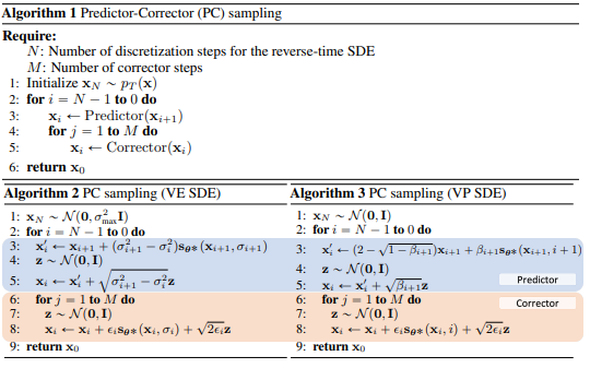
위에서 말한 reverse diffusion sampler와 같은 numerical한 방법만을 이용할 수도 있겠지만, 또 기존에 score-based model에서 활용하던 Langevin MCMC와 같은 method도 사용할 수 있다는 것을 까먹으면 안 된다. 그래서 저자는 이 두 가지를 Predictor-corrector method와 상응하는 방식으로 모두 적용하고자 하였고, 이를 Predictor-Corrector Sampler, PC sampler라 부른다. 좀 더 구체적으로는, numerical SDE Solver를 이용해 다음 time step의 sample을 얻고 (Predictor 역할) Langevin MCMC 방식으로, 얻었던 sample을 수정한다 (Corrector 역할). 예를 들어 reverse diffusion sampler를 predictor로, annealed Langevin MCMC approach를 corrector로 채택할 수 있겠다. 기존의 SMLD는 predictor는 identity, corrector는 annealed Langevin MCMC, 즉 Corrector-only case라 볼 수 있다. 또한 기존의 DDPM은 predictor는 ancestral sampler, corrector는 identity, 즉 Predictor-only case라 볼 수 있겠다. Appendix G에 pseudo code로 PC sampling에 대한 자세한 설명이 있다. Algorithm 1이 PC sampling의 큰 틀이고, Algorithm 2,3이 위에 예시로 든 경우에서의 방식이다.

그렇다면 이 방식이 단순히 기존의 ancestral sampling이나 앞서 제안했던 reverse diffusion sampling을 적용한 것에 비해 어떤 성능을 보이는지 실험 결과를 봐야 되는데, 실험 결과 표에 probability flow라는 predictor를 적용한 결과도 있어서 우선 probability flow 내용과 Architecture 변경 사항들을 정리하고 실험 결과를 살펴보자.

Probability flow ODE

$d\mathbf{x}=\mathbf{f}(\mathbf{x},t)dt+g(t)d\mathbf{w}$로 주어지는 모든 diffusion process에 대해서, SDE와 같은 solution을 가지는 상응하는 deterministic process가 다음과 같은 ODE로 주어지고, 이를 probability flow ODE라고 부른다. ODE를 NN을 통해 (정확히는 ODE coefficient 중 score를) 해를 구하는, ODE-Net의 예시라 볼 수 있겠다. 그래서 우리는 요 식을 통해서 input data distribution을 ODE Solver를 이용하여 구할 수 있게 되었다.

\[d\mathbf{x}=[\mathbf{f}(\mathbf{x},t)-\frac{1}{2}g(t)^{2}\nabla_{\mathbf{x}}log\;p_{t}(\mathbf{x})]dt\]

Appendix D

그럼 어떻게 해서 저 식이 튀어나오게 되었는가. 기본적으로는 [Fokker-Plank Equation]을 이용한다.

\[\begin{align*} \frac{\partial p_{t}(\mathbf{x})}{\partial t}&=-\sum_{i=1}^{d}\frac{\partial }{\partial x_{i}}[f_{i}(\mathbf{x},t)p_{t}(\mathbf{x})]+\frac{1}{2}\sum_{i=1}^{d}\frac{\partial }{\partial x_{i}}\big[\sum_{j=1}^{d}\frac{\partial }{\partial x_{j}}[\sum_{k=1}^{d}G_{ik}(\mathbf{x},t)G_{jk}(\mathbf{x},t)p_{t}(\mathbf{x})]\big] \\ &=-\sum_{i=1}^{d}\frac{\partial }{\partial x_{i}}[f_{i}(\mathbf{x},t)p_{t}(\mathbf{x})] \\ &+\frac{1}{2}\sum_{i=1}^{d}\frac{\partial }{\partial x_{i}}\big[p_{t}(\mathbf{x})\nabla \cdot [\mathbf{G}(\mathbf{x},t)\mathbf{G}(\mathbf{x},t)^{T}]+p_{t}(\mathbf{x})\mathbf{G}(\mathbf{x},t)\mathbf{G}(\mathbf{x},t)^{T}\nabla_{\mathbf{x}}log\,p_{t}(\mathbf{x})\big] \\ &(\because \frac{\partial p_{t}(\mathbf{x})}{\partial x_{j}}=p_{t}(\mathbf{x})\frac{\partial }{\partial x_{j}}log\,p_{t}(\mathbf{x})) \\ &=-\sum_{i=1}^{d}\frac{\partial }{\partial x_{i}}\Big\{f_{i}(\mathbf{x},t)p_{t}(\mathbf{x}) \\ &-\frac{1}{2}\big[\nabla \cdot [\mathbf{G}(\mathbf{x},t)\mathbf{G}(\mathbf{x},t)^{T}]+\mathbf{G}(\mathbf{x},t)\mathbf{G}(\mathbf{x},t)^{T}\nabla_{\mathbf{x}}log\,p_{t}(\mathbf{x})\big]p_{t}(\mathbf{x}) \Big\} \\ &=-\sum_{i=1}^{d} \frac{\partial }{\partial x_{i}}[\tilde{f_{i}}(\mathbf{x},t)p_{t}(\mathbf{x})] \\ &where\; \tilde{\mathbf{f}}(\mathbf{x},t):=\mathbf{f}(\mathbf{x},t)-\frac{1}{2}\nabla \cdot [\mathbf{G}(\mathbf{x},t)\mathbf{G}(\mathbf{x},t)^{T}]-\frac{1}{2}\mathbf{G}(\mathbf{x},t)\mathbf{G}(\mathbf{x},t)^{T}\nabla_{\mathbf{x}}log\,p_{t}(\mathbf{x})\end{align*}\]

맨 마지막 두 식을 보면, G가 0이고 drift term이 \(\mathbf{f}\)가 아닌 \(\tilde{\mathbf{f}}\)인 SDE의 Fokker-Plank Equation과 동일하다. 그래서 위와 같은, 상응하는 flow ODE가 나오게 되었다.

그래서 initial data distribution을 ODE Solver를 이용해 아래와 같이 구할 수 있다. 실험에서는 NLL Test(atol=1e-5, rtol=1e-5)를 위해 scipy에서 제공하는 RK45 ODE Solver를 이용했다고 한다. 좀 더 정확히는, Appendix C에서 다룬 issue들로 인해 initial data (t=0)이 아니라 \(\epsilon=10^{-5}\)에서의 data distribution을 구한 것이라고 한다.

\[log\,p_{0}(\mathbf{x}(0))=log\,p_{T}(\mathbf{x}(T))+\int_{0}^{T}\nabla \cdot \tilde{\mathbf{f}_{\theta}}(\mathbf{x}(t),t)dt\]

혹은 앞서 했던 것 처럼 discretize 하여 sampling process를 진행할 수도 있다.

\[\begin{align*} \mathbf{x}_{i}&=\mathbf{x}_{i+1}-[\mathbf{f}_{i+1}(\mathbf{x}_{i+1})-\frac{1}{2}g_{i+1}^{2}s_{\theta^{*}}(\mathbf{x}_{i+1}, i+1)] \\ &=\mathbf{x}_{i+1}+\frac{1}{2}(\sigma_{i+1}^{2}-\sigma_{i}^{2})s_{\theta^{*}}(\mathbf{x}_{i+1}, i+1)\;\;(\mathrm{SMLD}) \\ &= (2-\sqrt{1-\beta_{i+1}})\mathbf{x}_{i+1}+\frac{1}{2}\beta_{i+1}s_{\theta^{*}}(\mathbf{x}_{i+1}, i+1)\;\;(\mathrm{DDPM}) \end{align*}\]

Architecture

기본은 DDPM의 구조를 그대로 따라간다고 한다. DDPM에서 모델 아키텍쳐는 Wide ResNet 기반 U-Net이 기본 base이고, weight normalization 대신 group normalization, 그리고 2개의 conv layer 사이에 self-attention block이 추가된 구조이다. diffusion time embedding은 Transformer의 sinusoidal position embedding을 활용했다. 그리고 EMA를 사용했었다. 여기서 SDE 저자들의 변경 사항은, Appendix H.1에 정리되어 있는데, StyleGAN-2에서의 사항들을 많이 적용한 것 같다. 전체적으로는 network depth를 증가시켰다고 보면 될 것 같다.

Experiment Results

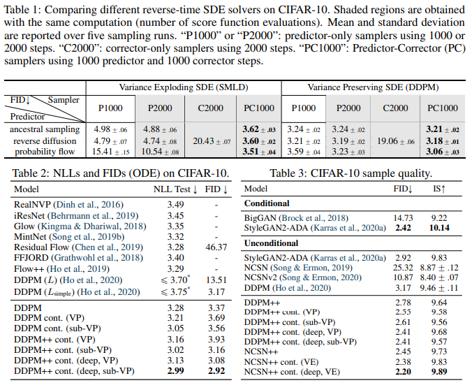
우선 Table 1은 CIFAR-10 dataset에서, ancestral sampler, reverse diffusion sampler, probability flow(Blackbox ODE Solver를 사용한 게 아니라 ODE를 discretization한 방식) sampler의 성능 비교와 Predictor-Corrector Sampling 방식의 성능 향상 여부를 SMLD 모델과 DDPM 모델 모두에게서 실험하였다. SMLD C2000은 기존 NCSN 모델이 되겠고, DDPM P1000/P2000은 기존 DDPM 모델이 되겠다. 표에서 알 수 있는 사실은

1. Reverse diffusion sampling은 ancestral sampling보다 항상 performance가 좋다.
2. Corrector-only는 다른 Predictor-only나 Predictor-Corrector 방식보다 performance가 좋지 않다. (performance가 비슷하기 위해서는 noise scale당 corrector step이 2번이 아니라 훨씬 더 많이 필요한데, 이는 computational cost를 높이는 것이라고 지적하고 있다.)
3. P1000과 PC1000을 비교하면, computation은 2배이지만 performance는 PC1000이 항상 좋다.
4. P2000과 PC1000을 비교하면, computation은 동일한데 performance는 PC1000이 항상 좋다.

그래서 결과적으로는 “Reverse diffusion sampling, Langevin MCMC sampling을 Predictor-Corrector mechanism으로 적용하면 best performance를 이끌 수 있다.”가 결론이 되겠다.

참고로 OpenReview에 있던 한 질문인데, 기존 NCSN 모델이 그럼 FID가 20이 넘을 만큼 왜 이렇게 안 좋게 나오느냐에 대한 질문이었다. 본문에 noise level 1000으로 실험했다는 말이 없어서 2000 step이 무슨 뜻인지 모를만하다. 이에 대한 해답은 기존 NCSN은 하나의 noise level에 대해서 여러 번에 거쳐 annealed Langevin step을 거쳤지만, 위 실험에서는 noise scale 당 2번의 corrector step (그래서 noise scale 1000x2=2000 step이라 C2000)을 거친 결과라고 한다. 실제로 C1000인 경우 FID가 39.2로 20.4인 C2000 보다 훨씬 높게(안 좋게) 나온다고 말했다.

Table 2는 CIFAR-10 dataset에서 Probability Flow ODE, ODE Solver를 이용했을 때의 결과를 보여주고 있다. 표에서 알 수 있는 사실은

1. 같은 DDPM 모델에서 input distribution을 exact하게 구할 수 있기에 bits/dim이 낮아졌다. (3.28)
2. 같은 DDPM 모델에서 objective를 continuous하게 바꾸었기에 bits/dim이 낮아졌다. (3.21)
3. sub-VP SDE가 VP SDE보다 bits/dim이 낮다.
4. Architecture 변경 사항이 bits/dim을 더 낮게 만들어주었다.

그런데 결과적으로는 “ODE Sampling 방식은 성능보다 sampling 속도 개선 측면에서 좋은 모습을 보였다”는 점을 알면 될 것 같다. Table 3를 보면 되는데.

Table 3는 CIFAR-10 dataset에서 앞선 모든것들을 적용해본 결과를 보여주고 있다. 변경한 architecture를 적용하고, PC sampler를 이용해 얻은 결과인데. 알 수 있는 사실은

1. VE SDE가 VP/sub-VP SDE 보다 FID socre가 낮다. 그러나 표에는 나와있지 않지만, VE SDE가 VP/sub-VP SDE보다 likelihood, bits/dim은 더 높게 나온다고 한다. trade-off 느낌.
2. FID=2.20의 최고 성능을 보인 NCSN++ cont. (deep, VE)는 기존의 conditional generative model보다도 더 낫다고 한다…

그래서 결과적으로는 “저자가 변경한, network의 depth를 증가시킨 모델에서 VE SDE를 위한 score matching 방식으로 학습하고, reverse inference 시에는 PC sampling을 활용하였다.”를 이해하면 될 것 같다.

4. Controllable Generation

Guided Diffusion 이후 여타 논문들에서 자주 보이는, class condition이 있을 때의 생성도 역시 이 framework에 적용될 수 있다. \(p_{0}\)의 sample이 아닌, \(p_{0}(\mathbf{x}(0)\mid \mathbf{y})\)의 sample. 우선 classifier가 학습되어 있어 \(p_{t}(\mathbf{y} \mid \mathbf{x}(t))\)를 안다고 가정하는데, classifier free guidance에서 했던 방식도 동일하게 적용 가능해 추가적인 학습이 필요 없다고 생각해도 된다. (Appendix I.4에 이에 대한 설명이 있다.) 기존과 동일하게 \(p_{T}(\mathbf{x}(T)\mid \mathbf{y})\)로 부터 아래의 conditioned reverse SDE를 풀면 initial conditioned distribution를 알 수 있다.

\[\begin{align*} d\mathbf{x}&=\{\mathbf{f}(\mathbf{x},t)-g(t)^{2}[\nabla_{\mathbf{x}}log\;p_{t}(\mathbf{x}\mid \mathbf{y})]\}dt+g(t)d\overline{\mathbf{w}} \\ &=\{\mathbf{f}(\mathbf{x},t)-g(t)^{2}[\nabla_{\mathbf{x}}log\;p_{t}(\mathbf{x})+\nabla_{\mathbf{x}}log\;p_{t}(\mathbf{y}\mid \mathbf{x})]\}dt+g(t)d\overline{\mathbf{w}} \end{align*}\]

5. Summary

Forward SDE: \(d\mathbf{x}=\mathbf{f}(\mathbf{x},t)dt+g(t)d\mathbf{w}\)

Reverse SDE: \(d\mathbf{x}=[\mathbf{f}(\mathbf{x},t)-g(t)^{2}\nabla_{\mathbf{x}}log\;p_{t}(\mathbf{x})]dt+g(t)d\overline{\mathbf{w}}\)

Corresponding Probability flow ODE: \(d\mathbf{x}=[f(\mathbf{x},t)-(1/2)g(t)^{2}\nabla_{\mathbf{x}}log\;p_{t}(\mathbf{x})]dt\)

우선, 기존의 Score-Matching based model과 Diffusion based model 모두가 “Solve SDE”라는 framework로 설명될 수 있음을 보였다. 또한 기존의 Diffusion model은 computationally expensive한 ancestral sampling 방식으로 reverse DE를 풀어서 데이터를 생성해냈으나, 본 논문에서는 reverse SDE를 PC(predictor-corrector) sampler를 제시하여 생성 모델의 성능 개선을 보였고, deterministic sampler(Probability Flow ODE)를 제시해 더 빠른 sampling을 할 수 있도록 하였다.

이후에는 더 좋은 reverse SDE/ODE integrator는 무엇인가에 대한 연구들이 이어지게 된다. [Zhang & Chen, 2022] [Lu et al., 2022] [Karras et al., 2022]

Reference

Papers

[1] Song, Y., Sohl-Dickstein, J., Kingma, D. P., Kumar, A., Ermon, S., & Poole, B. (2020). Score-based generative modeling through stochastic differential equations. arXiv preprint arXiv:2011.13456.