[Review] ODE/SDE-Net

Neural Network를 좀 더 다른 시각으로 바라볼 수 있게 한, ODE-Net과 그 variant인 SDE-Net에 대해 알아보자.

ODE-Net

기존의 ResNet은 $h_{t+1}=h_{t}+f(h_{t}, \theta_{t})$라는 형태로 나타내어 vanishing gradient 문제를 해결하였었다. 해당 식의 형태를 다른 관점으로 보면, ODE를 수치적으로 푸는 Euler method의 형태와 매우 유사하게 생겼다: $y_{n+1}=y_{n}+h\,f(t_{n},y_{n})$

그렇다면 layer를 더 촘촘하게 하고 step size를 더 작게 하면 discrete한 식이 아니라 Euler method처럼 continuous하게 되면서 network의 함수 f에 의해 결정되는 ODE, 다시 말해 $\frac{dh}{dt}=f(h(t),t,\theta)$를 만족하게 되지 않을까? 하는 것이 저자의 아이디어이다. 그래서 network의 output을 ODE IVP의 solution으로 보고 기존의 잘 알려진 ODE Solver를 이용해 output을 구한다. ODE Solver로는 Euler method를 포함해 Runga-Kutta, Midpoint, DOPRI, Adams–Bashforth 등 여러 가지가 있고 구현되어있다. 이렇게 하면 testing 시에 RNN과 같은 network를 하나하나 통과할 필요가 없고 ODE만 풀면 되기에 더 빠르다는 장점이 있다. (다만 RNN에 비해 학습이 조금 더 느리다고 한다.)

아래의 Pytorch implementation을 살펴보면 이해가 된다. 저자의 공식 github 레포에서 가져왔다.

    # 일부만 발췌.
    # https://github.com/rtqichen/torchdiffeq/tree/master
    class ODEfunc(nn.Module):

        def __init__(self, dim):
            super(ODEfunc, self).__init__()
            self.norm1 = norm(dim)
            self.relu = nn.ReLU(inplace=True)
            self.conv1 = ConcatConv2d(dim, dim, 3, 1, 1)
            self.norm2 = norm(dim)
            self.conv2 = ConcatConv2d(dim, dim, 3, 1, 1)
            self.norm3 = norm(dim)
            self.nfe = 0

        def forward(self, t, x):
            self.nfe += 1
            out = self.norm1(x)
            out = self.relu(out)
            out = self.conv1(t, out)
            out = self.norm2(out)
            out = self.relu(out)
            out = self.conv2(t, out)
            out = self.norm3(out)
            return out

    class ODEBlock(nn.Module):

        def __init__(self, odefunc):
            super(ODEBlock, self).__init__()
            self.odefunc = odefunc # 위에 정의된 네트워크 함수
            self.integration_time = torch.tensor([0, 1]).float()

        def forward(self, x):
            self.integration_time = self.integration_time.type_as(x)
            out = odeint(self.odefunc, x, self.integration_time, rtol=args.tol, atol=args.tol) 
            # odeint: RK4나 AdamsBashforthMoulton 과 같은 ODESolver
            return out[1]

        @property
        def nfe(self):
            return self.odefunc.nfe

        @nfe.setter
        def nfe(self, value):
            self.odefunc.nfe = value
    

기존 ResNet의 CNN layer에서 살짝의 변형이 있긴 하지만 거의 비슷한 형태로 ODE 속 함수 f를 구성하였고 이를 forward 할 때는 RK4와 같은 ODE solver를 이용해 output을 구하게 되는 것이다. 학습도 거의 비슷하게 아래와 같이 진행된다. MNIST dataset에서의 performance를 확인하는 코드에서 가져왔다.

    # 일부만 발췌.
    # https://github.com/rtqichen/torchdiffeq/tree/master
    feature_layers = [ODEBlock(ODEfunc(64))] if is_odenet else [ResBlock(64, 64) for _ in range(6)]

    model = nn.Sequential(*downsampling_layers, *feature_layers, *fc_layers).to(device)

    criterion = nn.CrossEntropyLoss().to(device)
    optimizer = torch.optim.SGD(model.parameters(), lr=args.lr, momentum=0.9)

    optimizer.zero_grad()
    x, y = data_gen.__next__()
    logits = model(x)
    loss = criterion(logits, y)
    loss.backward()
    optimizer.step()

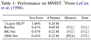
여기서 RK-Net은 ODE-Net과 architecture는 동일한데 Runge-Kutta integrator의 계산 방식을 그대로 역으로 따라서 backpropagation한 network이다. Backprop을 진행하기 위해 activation들을 저장해야 되어 Memory가 $O(\widetilde{L})$ (이 때 $\widetilde{L}$ 은 RK4에서 필요한 연산 수)인데, 그럼 ODE-Net은 Backprop을 어떻게 진행하기에 Memory가 constant인 것인가.

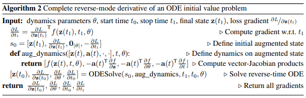
Forward는 ODE Solver를 이용했다면, Backprop을 통한 model의 parameter update 방식은 어떻게 되는가? 에 대한 의문을 해결하는 방법으로 adjoint sensitivity method를 사용한다. Loss function L에 ODE Solver의 output을 넣은 최종 Loss $L(ODESolver(z(t_{0}),f,t_{0},t,\theta))$로 부터 우리는 $\frac{\partial L}{\partial \theta}$를 알아야 된다. 이 때, adjoint라 불리는 $a(t):=\frac{\partial L}{\partial z(t)}$를 도입하면 \(\frac{\partial L}{\partial \theta}=-\int_{t_{0}}^{t}a( \tau)^{T}\frac{\partial f(z( \tau),\tau,\theta)}{\partial \theta}d \tau\)를 통해 우리의 목표를 달성할 수 있다. 그리고 adjoint는 $\frac{\mathrm{d} a}{\mathrm{d} t}=-a(t)^{T}\frac{\partial f(z(t),t,\theta)}{\partial z}$ 라는 또 다른 ODE를 만족 (Appendix B.1에 proof가 있다. 그냥 미분 정의 쓴 간단한 형태이다)해서 ODE Solver를 돌림으로써 Backpropagation을 할 수 있게 된다. 마찬가지로 start time $t_{0}$와 end time $t$에 대한 gradient도 구할 수 있다 (Appendix B.2). 이 방법의 좋은 점은 ODE Solver의 계산을 따라서 하지 않기 때문에 activation을 저장할 필요가 없어서 메모리와 시간 모두를 줄일 수 있다.

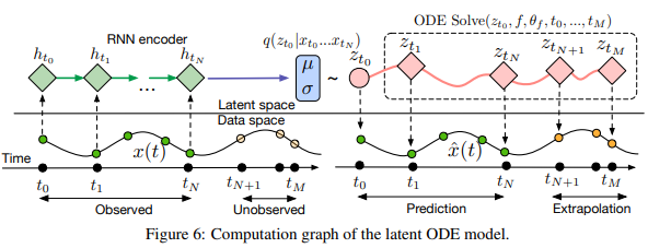
ODE-Net의 특성상 자연스럽게 time-series data를 다루는 걸 고려해볼 수 있는데, 논문에서는 RNN을 encoder로, ODE-Net을 decoder로 하는 VAE를 이용한 생성 모델을 구성하였다. Encoder에서 posterior를 샘플링한 것을 ODE Solver을 이용해 latent trajectory를 얻고 이를 다시 data space로 보내는 형태. 자세하게 살펴보지는 않겠다.

Summary

Neural Network를 기존에는 hidden layer의 discrete sequence로 바라보았다면, 저자는 network output을 수치해석학에서 증명된 ODE solver를 접목하여 구하였다. 또한, backpropagation을 ODE solver의 계산을 따라 곧대로 하지 않고 adjoint sensitivity method을 이용해 또 다른 ODE를 풂으로써 backprop시 gradient을 효과적으로 구할 수 있도록 하였다.

SDE-Net

SDE란

Stochastic Differential Equation, SDE, 확률 미분 방정식이란 기존의 ODE와는 다르게 uncertainty를 포함하는 미분방정식이다. 가령 $dN(t)=\alpha N(t)$와 같은 ODE에서 $dN(t)=\alpha N(t)+Noise$ 처럼 noise를 추가하여 uncertainty를 보장해주는 것이다. 이 때 Noise는 알 수 없는 값이기에 Random process가 될 수 밖에 없다. 즉, SDE는 “ODE에 uncertainty를 보장하기 위해 Noise를 더해주는 것”, 혹은 그 자체로 “Random process의 DE”로 해석하면 되겠다.

그 중 논문에서 자주 등장하는 Stochastic Process는 Brownian Motion/Standard Brownian Motion/Wiener Process가 있다. (다 같은 거) 아래의 조건을 모두 만족하는 stochastic process를 Brownian Motion $W_{t}$이라 부른다.

1. $W_{0}=0$
2. $W_{t}-W_{s} \sim N(0,t-s) \forall t\geq s \geq 0$
3. For every pair of disjoint time intervals $[t_{1},t_{2}]$, $[t_{3},t_{4}]$, with $t_{1}<t_{2}\leq t_{3}<t_{4}$, $W_{t_{4}}-W_{t_{3}}$ and $W_{t_{2}}-W_{t_{1}}$ are independent random variables
4. $W_{t}$ is continuous, but not differentiable in almost anywhere

그랬을 때 Brownian motion을 기초로 하는 임의의 stochastic process에 대한 SDE는 다음과 같이 일반화 할 수 있다:\(dX_{t}=f(dX_{t},t)dt+g(dX_{t},t)dW_{t}\) (이 때, \(W_{t}\)는 Weiner Process). 이 때, \(f(dX_{t},t)\)는 시간의 흐름에 따라 확정적으로 변하는 양, 결정론적인 Part라 drift coefficient라 부르고, \(g(dX_{t},t)\)는 도저히 알 수 없는 변동, 확률론적인 Part라 diffusion coefficient라 부른다. 이렇게 drift term과 diffusion term이 time과 stochastic process에 의존하는 SDE를 Itô SDE라고 부르기도 한다.

2003년 Øksendal에 의해 증명된 바에 따르면, drift와 diffusion coefficient들이 time, state 모두에 대해 globally Lipschitz 하다면 SDE가 unique strong solution을 가진다고 한다.

SDE도 ODE와 마찬가지로 수치해석학적으로 시뮬레이션을 통해 해를 구하는 Solver가 있는데, 논문에서도 활용한 가장 간단하면서도 대표적인 방법은 Euler-Maruyama method이다. \(dX_{t}=f(dX_{t},t)dt+g(dX_{t},t)dW_{t}\)라는 SDE가 주어져있을 때 \(Y_{n+1}=Y_{n}+f(Y_{n}, \tau_{n})\Delta t+g(Y_{n}, \tau_{n})\Delta W_{n}\)의 Markov chain Y를 통해 true solution X를 구하는 방법이다. ODE에서의 Euler-method와 유사하면서도 뒤에 \(+g(Y_{n}, \tau_{n})\Delta W_{n}\) term이 추가적으로 붙은 형태이다. 이 때, \(\Delta W_{n}\)은 Brownian motion 정의에 의해 mean이 0이고 variance가 \(\Delta t\)인 정규분포이고, 실제 implementation은 Gaussian distribution에서 sampling을 하는 방식으로 하면 되겠다.

마찬가지로 SDE-Net의 저자 또한 ODE-Net의 uncertainty에 대해 지적하고 있다. 우선 uncertainty를 2가지 종류로 나누자면 Aleatoric Uncertainty(class overlap, data noise와 같은 자연적인 랜덤성)과 Epistemic Uncertainty(lack of observation data 처럼 학습되지 않은 데이터에서 나오는 랜덤성)가 있다. 기존에는 Bayesian 방법들 (BNN)이 주를 이루었는데 이는 prior를 도입함에 있어 이를 특정하기 어렵고, parameter가 많아 계산이 어렵다는 단점이 있다. Non-Bayesian 방법들은 model ensembling을 통해 uncertainty를 얻고자 하였으나, 여러 모델을 학습하는 것은 computational cost 측면에서 단점이 있다. ODE-Net을 떠올려보면, ODE 자체가 deterministic 하기 때문에 epistemic uncertainty를 model할 수 없다는 단점이 있어서 이를 극복하고자 neural SDE model을 구성하게 된 것이다.

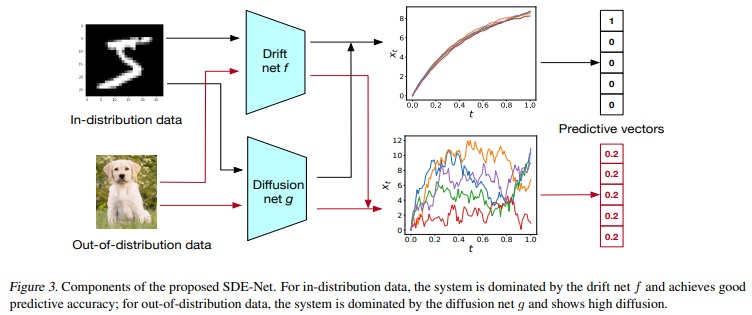
SDE-Net Model은 2개의 네트워크로 구성되어 있다. Drift Net f는 SDE의 drift term을 나타내는 network로, classification 시 좋은 예측 정확도를 학습하는 것을 목표로 한다. 또 다른 역할로는 aleatoric uncertainty를 capture하는 것이다. classification 시 mean을 출력해 Crossentropy로 학습한다. 그리고 Diffusion Net g는 SDE의 diffusion term을 나타내는 network로, (1) in-distribution(ID) data일 때에는 Brownian motion의 variance가 작아야 하므로 drift term에 의해 결정되도록 하고, (2) out-of-distribution(OOD) data일 때에는 variance가 커야 하므로 diffusion term에 의해 결정되도록 한다. classification 시 binary crossentropy로 학습해 OOD와 ID를 학습한다.

학습의 objective function을 보면 이해가 된다. \(\underset{\theta_{f}}{min} E_{x_{0}\sim P_{train}}E(L(x_{T}))+\underset{\theta_{g}}{min} E_{x_{0}\sim P_{train}}g(x_{0};\theta_{g})+\underset{\theta_{g}}{max} E_{\tilde{x_{0}}\sim P_{OOD}}g(\tilde{x_{0}};\theta_{g})\)

OOD input으로는 input에 Gaussian noise를 더하는 방법이 있고, 혹은 다른 종류의 데이터를 사용할 수도 있다. 아무튼 training data로 loss를 최소화 함과 동시에 ID data에 대해서는 diffusion net이 low diffusion을 출력하도록 학습하면서 OOD data에 대해서는 diffusion net이 high diffusion을 출력하도록 학습한다.

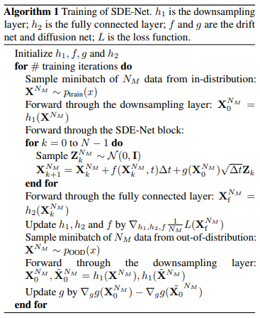
1. ID data에서 minibatch를 sampling 해서 downsampling layer를 통과한다.
2. Drift net f와 Diffusion net g를 통과시킨 값을 Euler-Maruyama method를 이용하여 N번의 step을 거친다.
3. FC layer를 거친다.
4. Loss를 구하여 downsampling layer, FC layer, drift net을 update한다.
5. OOD data에서 minibatch를 sampling 해서 downsampling layer를 통과한다.
6. Binary Cross-entropy로 diffusion net을 학습한다. ID minibatch는 true label, OOD minibatch는 fake label을 준다.

Reference

Websites

[사이트 출처 1] (https://seewoo5.tistory.com/12)

[사이트 출처 2] Wikipedia: Stochastic differential equation, Itô calculus, Euler–Maruyama method, Wiener process

Papers

[1] Chen, R. T., Rubanova, Y., Bettencourt, J., & Duvenaud, D. K. (2018). Neural ordinary differential equations. Advances in neural information processing systems, 31.

[2] Kong, L., Sun, J., & Zhang, C. (2020). Sde-net: Equipping deep neural networks with uncertainty estimates. arXiv preprint arXiv:2008.10546.