[Review] NCSN
앞서 Review한 diffusion model이 그냥 툭하고 튀어나온게 아니다. 사실 Diffusion Model은 score-based model을 diffusion probabilistic model에 통합한 모델로써 의미가 있는데, 이를 이해하기 위해 Score-based model과 관련된 논문들을 살펴보자. Yang Song 씨의 논문의 대다수이다.
- Estimation of Non-Normalized Statistical Models by Score Matching
- A Connection Between Score Matching and Denoising Autoencoders
- Generative Modeling by Estimating Gradients of the Data Distribution (NCSN)
- Improved Techniques for Training Score-Based Generative Models (NCSNv2)
0. Introduction
Stochastic Gradient Langevin Dynamics (SGLD)
딥러닝 학습에 있어서 parameter update하는 것을 생각해보자. $X$라는 N개 dataset이 주어져있을 때, 우리의 궁극적인 목표는 실제 데이터의 분포 $p_{X}(.)$를 model parameter $\theta$를 통해 $p(\theta \mid X)$, 다시 말해 X가 주어졌을 때 그 분포, pdf를 학습하는 것이다. $p(\theta \mid X) \propto p(\theta)\prod_{i=1}^{N}p(x_{i}\mid \theta)$ 이기에 optimization은 $argmax \; p(\theta)\prod_{i=1}^{N}p(x_{i}\mid \theta)$, MAP(Maximum a posteriori)를 찾으면 되는 것이다. $argmax \; log\;p(\theta)+\sum_{i=1}^{N}log\;p(x_{i}\mid \theta)$와 같겠다.
잘 알려져있는, 모두가 쓰는 방법은 Gradient Descent(GD), 특히 Stochastic Gradient Descent(SGD) 방법으로 전체 dataset X의 subset(=minibatch)에 대해서 $\Delta \theta_{t}=\frac{\epsilon_{t}}{2}(\nabla_{\theta_{t}}log p(\theta_{t})+\frac{N}{n}\sum_{i=1}^{n}\nabla_{\theta_{t}}log p(x_{i,t}\mid \theta_{t}))$로 파라미터을 업데이트한다. $\epsilon_{t}$는 step size, decreasing 하고 summation이 무한대이며 energy(square sum)는 finite한 조건이 붙어야 수렴한다.
여기서 SGLD의 논문에서는, 이런 SGD 방식이 parameter uncertainty를 놓쳐서 overfitting의 가능성이 있기에 이런 uncertainty를 capture하기 위한 Bayesian approach로 Markov chain Monte Carlo(MCMC) tech., 그 중에서도 Langevin dynamics를 소개하고 있다. gradient step 뿐만 아니라 Gaussian noise를 parameter update 시에 추가해주는 것. SGLD는 이런 Langevin Dynamics를 SGD와 합쳐서 업데이트 하는 방식을 제안했다. 즉, $\Delta \theta_{t}=\frac{\epsilon_{t}}{2}(\nabla_{\theta_{t}}log p(\theta_{t})+\frac{N}{n}\sum_{i=1}^{n}\nabla_{\theta_{t}}log p(x_{i,t}\mid \theta_{t}))+\epsilon_{t}\eta_{t} \quad where \; \eta_{t}\sim N(0,I)$. $\Delta \theta_{t} \sim N(\frac{\epsilon_{t}}{2}(\nabla_{\theta_{t}}log p(\theta_{t})+\frac{N}{n}\sum_{i=1}^{n}\nabla_{\theta_{t}}log p(x_{i,t}\mid \theta_{t})), \epsilon_{t}I)$와 같은 말이다.
사실 SGLD를 optimization으로 소개하긴 했지만, Langevin MCMC 자체는 Bayesian learning에서 sampling에서도 쓰인다. \(\widetilde{x}_{T}=\widetilde{x}_{T-1}+\frac{\epsilon}{2}\nabla_{x}log\,p(\widetilde{x}_{T-1})+\sqrt{\epsilon}z_{T}\;where\;z_{T}\sim N(0,I)\).
잠시 DDPM으로 돌아가보자면, DDPM의 Abstract에 보면 이런 문장이 나온다.
desinged according to a novel connection between diffusion probabilistic models and denoising score matching with “LANGEVIN DYNAMICS”
denoising score matching은 아래에서 다루고, 여기서 말하는 Langevin dynamics가 결국 backward sampling에 있어 $x_{t-1}=\frac{1}{\sqrt{\alpha_{t}}}(x_{t}-\frac{1-\alpha_{t}}{\sqrt{1-\overline{\alpha_{t}}}}\epsilon_{\theta}(x_{t},t))+\sqrt{\sigma_{t}}z$ 했던 행동이 Langevin MCMC와 유사한 형태임을 알 수 있다. (scale factor가 추가된 정도이다)
요 Langevin Dynamics를 활용한 Sampling은 NCSN을 다룰 때 튀어나올 예정이다.
Energy-Based Model
Energy function을 통해 pdf를 정의하고, 이를 통해 실제 데이터의 분포를 예측하고자 했던 모델이다. 다시 말해 energy function을 학습하는 것을 목표로 하는 모델. $X$라는 N개 dataset이 주어져있을 때, Energy function을 $\epsilon_{\theta}(x)$로 정의한다면 이것을 가지고 Boltzmann distribution을 통해 pdf를 정의할 수 있다: $p_{\theta}(x)=\frac{exp(-\epsilon_{\theta}(x))}{Z(\theta)}$. 이 때 $Z(\theta)=\int exp(-\epsilon_{\theta}(x))dx$는 normalizing coefficient. 이 논문에서도 파라미터를 업데이트함에 있어 SGLD를 사용하는데, $\nabla_{\theta_{t}}log \;p_{\theta_{t}}(x)=\nabla_{\theta_{t}}\epsilon_{\theta_{t}}(x)-\nabla_{\theta_{t}}log\;Z(\theta_{t})$로 정리된다.
1. Score-Matching
Energy-Based Model의 문제점
간략히 소개한 EBM의 문제점에 대해 크게 2가지 정도로 설명하고 있다.
- 적분 형태로 주어지는 $Z_{\theta}$는 analytically intractable한 경우가 대다수이다. 즉, 학습 시에 $-\nabla_{\theta_{t}}log\;Z(\theta_{t})$는 analytically & numerically 계산 불가능하다.
- $\nabla_{\theta_{t}}\epsilon_{\theta_{t}}(x)$는 모델을 학습시키는거라 pytorch가 알아서 해줄건데, $-\nabla_{\theta_{t}}log\;Z(\theta_{t})$는 어떻게 되는가. EBM의 논문에서 이를 정리하면 $\nabla_{\theta_{t}}log\;Z(\theta_{t})=E_{x \sim p_{\theta_{t}}(x)} [ -\nabla_{\theta_{t}}\epsilon_{\theta_{t}}(x)]$가 된다고 적혀있다. 이걸 자세히 보면, $p_{\theta_{t}}(x)$에서 sampling을 해야 되는데, 이 자체가 오래 걸릴 뿐더러 학습한 모델에서 또 추가적인 연산이 필요하다. 본 논문에서는 “Estimation of non-normalized models is approached by MCMC methods, which are VERY SLOW, or by making some approximations, which may be quite poor”라고 말하고 있다.
개선점
Main idea는 “$p_{\theta}(x)$가 아닌 $s_{\theta}(x):= \nabla_{x} log\; p_{\theta}(x)$를 학습하는 것, 즉 그냥 density가 아닌 gradient of log-density”이다. score function이라고 말하는 것도 gradient of log-density이다. 이렇게 했을 때의 장점은, $\nabla_{x} log\;p_{\theta}(x)=-\nabla_{x}\epsilon_{\theta}(x)$로, $Z(\theta)$에 대한 걱정이 사라진다는 점.
그랬을 때 model의 목표는 단순 regression task 처럼 model score function과 실제 data의 score function간의 distance를 최소화 하는 것이다. 다시 말해, \(J(\theta)=\frac{1}{2} \int p_{data}(x)\|s_{\theta}(x)-\nabla_{x}log \; p_{data}(x)\|_{2}^2dx \\ =\frac{1}{2}E_{p_{data}}[\|s_{\theta}(x)-\nabla_{x}log \; p_{data}(x)\|_{2}^2]\) 가 되겠다. 따라서 이를 최소화하는 $argmin \; J(\theta)$가 우리의 최종 파라미터가 되겠다. 논문에서 Theorem 1으로, 해당 objective는 \(J(\theta)=\frac{1}{2}\int p_{data}(x) [ tr(\nabla_{x}s_{\theta}(x))+\frac{1}{2}\|s_{\theta}(x)\|_{2}^{2} ]dx \;+\;const \\ = \frac{1}{2}E_{p_{data}}[tr(\nabla_{x}s_{\theta}(x))+\frac{1}{2}\| s_{\theta}(x)\|_{2}^{2}]\;+\;const' \\ \approx \frac{1}{N}\sum_{i=1}^{N} [ tr(\nabla_{x_{i}}s_{\theta}(x_{i}))+\frac{1}{2}\|s_{\theta}(x_{i})\|_{2}^{2} ] \;+\;const''\)로 계산할 수 있으며, Theorem 2 및 Corollary 3으로 SGLD를 쓰면 큰 수의 법칙에 의해 $\nabla J(\theta)=0$이 되는 우리의 목표인 파라미터로 업데이트가 적절히 이루어진다고 말하고 있다.
여기에 있어서 score function이 미분 가능하고, weak regularity 조건 (data distribution $p_{data}(x)$가 미분 가능하고, model score function과 실제 data score function의 square의 expectation이 유한하며, data의 분포와 model score의 분포의 곱이 어떠한 파라미터에 대해서라도 무한히 큰 값에 대해 0으로 수렴한다), 그리고 data distribution과 일치해지는 파라미터가 유일하게 존재하는 가정이 들어간다. 좋은 상황을 가정하자는 거다. 그렇지 않다면 typical한 SGD 처럼 global minima가 아닌 local minima에 빠질 수 있고, unexpected behavior를 보일 수 있기에.
Example
논문의 Section 3.1에 Multivariate Gaussian Density를 예시로 앞서 말한 설명을 보여주고 있는데, 이걸 보니까 한 번에 확 와 닿았다. pdf로 Guassian density function, 파라미터 $\theta={M,\mu}$일 때 $p_{M,\mu}(x)=\frac{1}{Z(M,\mu)}exp(-\frac{1}{2}(x-\mu)^{T}M(x-\mu))$로 ground-truth data pdf인 Guassian pdf를 유추한다고 가정해보자. 물론 이 경우에 한정해서는 $Z(\theta)$가 무엇인지 널리 알려져있지만, 모른다고 가정해보자. (애초에 실제 데이터가 어떤 분포를 따르는지 조차 모르는 경우가 대다수이며, $Z(\theta)$를 아는 경우는 현실에 거의 없다) 그렇다면 score function은 $s_{\theta}(x):= \nabla_{x} log\; p_{\theta}(x)=-M(x-\mu)$가 될 것이고, $tr(\nabla_{x}s_{\theta}(x))=-\sum m_{ii}$가 되기에, $J(\theta)=\frac{1}{N}\sum_{i=1}^{N}[-\sum m_{jj}+\frac{1}{2}(x_{i}-\mu)^{T}MM(x_{i}-\mu)]\;+\;const$가 된다. (N개의 data point $x_{i}$들, $M^{T}=M$은 당연) 따라서, $\nabla J(\theta)=0$이 되는 파라미터를 찾으면 되는데, $\nabla_{\mu} J(\theta)=MM\mu-MM\frac{1}{N}\sum x_{i}$ 라서 0이 되는 건 $\mu=\frac{1}{N}\sum_{i=1}^{N} x_{i}$가 되겠고, $\nabla_{M} J(\theta)=-I+M\frac{1}{2N}\sum_{i=1}^{N}(x_{i}-\mu)(x_{i}-\mu)^{T}+\frac{1}{2N}[\sum_{i=1}^{N}(x_{i}-\mu)(x_{i}-\mu)^{T}]M$ 이라서 0이 되는 건 $M^{-1}=\frac{1}{N}\sum_{i=1}^{N}(x_{i}-\mu)(x_{i}-\mu)^{T}$가 되겠다. score matching 방식으로 찾은 평균과 분산이, Maximum likelihood Estimation 방법으로 찾은 평균/분산과 동일하다. 다시 생각해보면, 어떤 N개의 data가 있을 때 모집단의 평균은 당연히 sample average $\frac{1}{N}\sum_{i=1}^{N} x_{i}$ 로 추정할 것이고 분산은 당연히 sample covariance matrix $\frac{1}{N}\sum_{i=1}^{N}(x_{i}-\mu)(x_{i}-\mu)^{T}$의 inverse로 추정하게 되는 그 직관과 동일하며 우리가 원하는 결과를 score matching 방식으로도 얻게 되는 것이다. N이 크니까 모집단의 분산 N-1이나 N이나 뭐
Summary
결국 기억해둬야 될 것은 gradient of log-likelihood를 score로 정의해서, model score $s_{\theta}(x):= \nabla_{x} log\; p_{\theta}(x)$와 data score $\nabla_{x} log\; p_{data}(x)$를 일치시키는 (L2 loss) 것이다.
2. Denoising Score-Matching
기존 Score-Matching의 문제점
Score Matching의 objective를 다시 보자:\(J(\theta)\approx \frac{1}{N}\sum_{i=1}^{N} [ tr(\nabla_{x_{i}}s_{\theta}(x_{i}))+\frac{1}{2}\|s_{\theta}(x_{i})\|_{2}^{2} ] \;+\;const\) 여기서 \(\frac{1}{2}\| s_{\theta}(x)\|_{2}^{2}\) 부분은, model을 통과한 \(s_{\theta}(x)\)로 부터 바로 구해질 수 있으나, \(tr(\nabla_{x}s_{\theta}(x))\) 부분은, \(s_{\theta}(x)\)의 Jacobian matrix을 가지고 있어야 되기에 computational cost가 높다. 당연히 오래 걸리는 건 우리가 원하는 게 아니다.
본 논문에서 제시한 내용을 보기 전에, prerequisite으로 2가지 정도 알고 넘어가자.
Parzen Window Density Estimation
우리가 input으로 주는 data는 어떤 식으로 분포되어 있는지 일반적으로는 전혀 알 수 없다. 정규 분포를 띈다? 그건 매우 운이 좋은 케이스라 볼 수 있겠다. 이럴 때 데이터의 분포, pdf를 추정하는 방법으로는 Kernel density estimation 혹은 KNN 등 여러가지 방법이 있지만 해당 논문에서 density estimator를 언급하고 있다.
pdf $p(x)$를 estimate하기 위해서, density라는 게 일정한 범위 내에서 데이터가 몇 개 있는가를 나타내기 때문에 $p(x)\approx \frac {k}{NV}$임을 이용한다. 이 때 V는 범위, N은 전체 데이터 수, k는 해당 범위에 속한 데이터 수를 뜻한다. KNN은 K를 고정했을 때 V를 결정하는 것이라 볼 수 있겠고, Kernel method는 V를 고정했을 때 K를 결정하는 방식이라 볼 수 있겠다. k를 결정하는 kernel function $K(u)$는 여러 가지가 있는데, Parzen Window는 이런 kernel function들 중 하나로, 길이 h의 hypercube가 있을 때 그 안에 속해있는 데이터 수를 세는 것이다. D dimension에서 $V=h^{D}$, \(k=\sum_{i=1}^{N}K(\frac{x_{i}-x}{h}) \; where \; K(u) = 1_{A}(u),\; A=\{u=[u_{1},...,u_{D}]^{T} \mid \exists \, n \, s.t. \|u_{n}\|\leq \frac{h}{2}\}\) 가 되겠다. 또 다른 kernel function으로는 Gaussian kernel이 있으며, 논문에서는 Guassian kernel을 고려한다. 이유는 그냥 식이 간단해져서. 내가 알기로는 Parzen Window라는 kernel function이 있고 Gaussian kernel이라는 kernel function이 있다. 이렇게 알고 있는데 논문에서는 그냥 동일하게 본다.
Denoising Autoencoder
“Extracting and composing robust features with denoising autoencoders”라는 2008년 논문에서 처음으로 제시된 Denoising autoencoder는 되게 간단한 구조이다.
- Training input $x$를 그냥 넣지 않고, Gaussian noise를 추가한, $\widetilde{x}=x+\varepsilon, \; \varepsilon \sim N(0,\sigma^{2}I)$를 encoder의 input으로 준다.
- Encoder, Decoder를 통과하고 나온 output $x_{out}$을 기존 Autoencoder 처럼 Reconstruction error, L2 loss로 학습한다. 다만, $\widetilde{x}$가 아닌 $x$와 비교한다는 것.
어떻게 보면 VAE와 매우 유사하지만 latent 단이 아니라 input 단에서 noise를 넣고 있다. 또 어떻게 보면 2015년 처음으로 제시된 Diffusion Model과 “input에 noise를 넣고, 모델을 통과했을 때 기존 input과의 차이를 본다”는 점에서 비슷하지만, input에 noise를 여러 step에 걸쳐 계속 넣는 방향으로 발전한 것이라 볼 수 있겠다.
개선점
앞선 Score Matching 논문을 한 줄로 요약하자면, $J_{ESM_{q}} \sim J_{ISM_{q}} \sim \lim_{n\rightarrow \infty }J_{ISM_{q_0}}$이다. 다시 말해, data의 score와 model의 score간 matching인 Explicit Score Matching(ESM) 형태는 model score의 L2 norm과 trace of Jacobian의 조합으로 나타낸 Implicit Score Matching(ISM) 형태와 상수 차이이며, Finite Sample Version으로 구해도 적절한 가정과 Sampling을 계속할 시 동일한 결과를 얻는다.
우선, 기존의 ESM 형태인 \(J_{ESM_{q}(\theta)}=\frac{1}{2}E_{p_{data}}[\|s_{\theta}(x)-\nabla_{x}log \; p_{data}(x)\|_{2}^2]\; where \; s_{\theta}(x):= \nabla_{x} log\; p_{\theta}(x)\)에서 $p_{data}(x)$ 는 무엇일까. 앞서 말했듯이 input data의 distribution은 알면 운이 매우매우 좋은 경우라 했고, 일반적으로는 모르기 때문에 이를 Parzen window density estimator $p_{\sigma}(x)$로 추정했다고 가정하자. 이 때, Parzen window는 매우 좋은 함수(Score Matching 가정 조건에서의 weak regularity를 만족하는 함수)이기에, score matching에서 다룬 동일한 논리를 적용하면 이 estimator를 이용한 ESM과 ISM이 상수 차이가 된다. 즉, $J_{ESM_{p_{\sigma}}} \sim J_{ISM_{p_{\sigma}}}$.
그리고 대망의 Main idea는 Score Matching Principle과 Denoising Autoencoder approach를 합치는 것이다. Denoising Autoencoder의 input처럼 clean input과 noisy input pair $x,\widetilde{x} $가 있을 때, Joint density $p_{\sigma}(\widetilde{x})=p_{\sigma}(\widetilde{x} \mid x)p_{data}(x)$의 score를 고려해보자. 그렇다면 우리의 목표, Denoising Score Matching(DSM)은 \(J_{DSM_{p_{\sigma}}(\theta)}=\frac{1}{2}E_{p_{\sigma}(\widetilde{x})}[\|s_{\theta}(\widetilde{x})-\nabla_{\widetilde{x}}log \; p_{\sigma}(\widetilde{x})\|_{2}^2]\; where \; s_{\theta}(\widetilde{x}):= \nabla_{\widetilde{x}} log\; p_{\theta}(\widetilde{x})\)가 되겠다. 그랬을 때 Kernal Density Estimator $p_{\sigma}(\widetilde{x} \mid x)$를 Guassian Kernel을 사용한다면, $\nabla_{\widetilde{x}}log \; p_{\sigma}(\widetilde{x})$ 항은 $-\frac{x-\widetilde{x}}{\sigma^{2}}$로 간단해진다.
그리고 저자는 Appendiex에서 \(J_{DSM_{p_{\sigma}}} \sim J_{ESM_{p_{\sigma}}}\)를, Section 4.3에서 \(J_{DSM_{p_{\sigma}}} \sim J_{DAE_{\sigma}}\)를 수식 전개를 통해 보이고 있다. 사실 직관적인지는 모르겠는데 직관적으로는 noisy data score function을 보면 clean input과 noisy input의 차이로 구성되어 있기에, noisy input이 clean input으로 돌아가는 과정에 있어서 model의 score가 그것과 matching 되도록 해주는 것이다. 아무튼.
Summary
논문에서 애초에 Section 5 Discussion 앞부분에 Summary를 제공해줬다. \(J_{DSM_{q_{\sigma}}}=\frac{1}{2}E_{p_{data}}E_{q_{\sigma}(\widetilde{x} \mid x) \sim N(x,\sigma^{2}I)}[\|s_{\theta}(\widetilde{x})+\frac{x-\widetilde{x}}{\sigma^{2}}\|_{2}^2]\)
Putting together equations 8, 11, and 14, we can write, for $\sigma >0$, \(J_{ISM_{q_{\sigma}}} \sim J_{ESM_{q_{\sigma}}} \sim J_{DSM_{q_{\sigma}}} \sim J_{DAE_{\sigma}}\)
In summary, training the denoising autoencoder defined in section 2 is equivalent to performing score matching (explicit or implicit) with the energy function of Eq. 12 on Parzen density estimate $q_{\sigma}$.
Sliced Score Matching
Score Matching의 단점이었던 $tr(\nabla_{x}s_{\theta}(x))$ 부분을 보완하기 위한 또 다른 방법으로, 다른 저자는 다른 방법을 고안하였다. \(E_{p_v}E_{p_{data}}[v^{T}\nabla_{x}s_{\theta}(x) v +\frac{1}{2}\| s_{\theta}(x)\|_{2}^{2}]\)인데, 언뜻 보면 식이 더 복잡해진것 처럼 보이지만 그렇지 않다. $p_v$는 multivariable standard normal random vector이고, trace of Jacobian을 대신한 저 term은 pytorch가 대신 해줄 수 있게 되었다. 다만, 연산량이 약 4배 정도 증가한 게 단점으로 작용할 수 있겠다.
3. NCSN
Yang Song Blog 논문 저자의 Blog에 본인이 정리해둔 글이 있다! 직접 보고 많은 도움이 되었다.
기존 Denoising Score-Matching의 문제점
우리의 원래 목적은 original data distribution $p_{data}(x)$를 score를 통해 유추하는 것인데, 해당 방법은 true data distribution의 score가 아니라 noisy input의 score, joint density $p_{\sigma}(\widetilde{x} \mid x)p_{data}(x)$의 score와의 matching이기에 noise가 충분히 작지 않을 경우 원래의 목적과 멀어진다.
Naive Approach의 문제점
Section 3에서 저자는 이런 score-based matching concept를 generative modeling에 naive하게 곧바로 적용하기에는 2가지 걸림돌이 있다고 말하며 이에 대해 설명하고 있다.
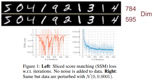
첫 번째로, Manifold Hypothesis이다. 그림에서 나와있듯이, 당장 MNIST만 해도 28*28=784 dimension에 있는 data를 595 dimension으로 줄여도 별 차이가 없음을 볼 수 있다. 이처럼 Real data는 ambient space/high dimensional space에서 low-dimensional manifold에 embedding 되어 있는 경향이 있다. 그렇다면, score-based model의 경우 score, true data distribution의 gradient of log density는 ambient space 상에서 계산되기에 기존에 있던 low-dimensional manifold에서 벗어날 수 있고, 애초에 data가 ambient space 전체에 분포되어 있지 않다면 consistent한 score estimator가 될 수 없다. 논문에서는 이를 실험을 통해 보였는데, Sliced Score Matching method로 CIFAR-10에서 생성모델을 학습할 때 loss가 감소하다가 fluctuating하는 모습을 볼 수 있었다. 즉, 현실 데이터에 score-matching generative model을 곧바로 적용하기에는 manifold hypothesis로 인해 학습이 불안정한 모습을 띈다는 것. 하지만 저자는 data에 $N(0,1e-4)$의 아주 작은 Gaussian noise를 더했을 때, loss가 converge하는 모습을 확인하였다. 이는 아주 작은 noise더라도 전체 data가 high-dimension에 고루 분포할 가능성을 높여주어 원래 바랬던 모습을 띄게 되는 것이며, 이것이 저자의 메인 idea가 된다.
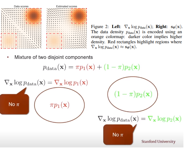
또한, Low density region에서 data의 부족이 Score estimation과 Langevin MCMC sampling 모두 어렵게 만든다. 상단의 그림이 논문에서 제시한 toy example인데, 사실 좀 당연하게 확률 분포 상 0에 가까워서 데이터가 거의 없는 경우 모델이 score를 학습하기는 어렵다. 그리고 하단의 그림이 Sampling에서의 obstacle을 보여주는데, score, 즉 gradient of log-likelihood의 정의 상 어떤 두 분포의 disjoint 합으로 표현된 분포가 있을 경우 그들의 상대적인 weight 정보가 score상에서 고려될 수 없다는 단점이 있다. Sampling을 해도 분포를 정확히 구할 수 없다는 말이다. 그렇다면 앞서 저자가 실험했던, Guassian noise를 더하면 이 문제점은 어떻게 될까? 전체 data가 high-demension에 고루 분포한다는 것은 low density region에도 data가 분포할 가능성이 증가한다는 뜻이기에 이 문제점 또한 해결할 수 있게 된다.
개선점
Main idea는 앞서 잠깐 말했듯이 Gaussian noise를 더해주는 것이다. 그러나 Denoising Score Matching에서 봤다 싶이 noise가 매우 작지 않을 경우 모델이 원래의 분포와 멀어지고, 그렇다고 noise를 작게 하면 앞서 말한 장점들을 충분히 이용할 수 없으니, 어떻게 해야 될까? 이에 대한 해답이자, 가장 Main이라고 볼 수 있는 idea는 “Multiple Level” of Gaussain noise를 사용하는 것이다. 하나의 모델에서 여러 개의 noise level에 해당하는 score를 전부 학습하고, inference 시에 large noise에서부터 noise level을 차차 줄여가며 sample를 얻는 것이다.
NCSN
$\sigma_{i}$가 $\frac{\sigma_{1}}{\sigma_{2}}=…=\frac{\sigma_{L-1}}{\sigma_{L}}>1$를 만족하는 noise들이라고 하자. 다시 말해 $\sigma_{1}$는 충분히 큰 noise로 앞서 말한 manifold hypothesis나 score matching에서의 문제점을 해결할 수 있도록 하면서도 $\sigma_{L}$은 충분히 작은 noise로 기존 clean data distribution과 거의 일치할 수 있도록 하는 sequence를 고려하자. 그리고 \(q_{\sigma}(x):=\int p_{data}(t)N(x \mid t, \sigma^{2}I)dt\) 의 perturbed data distribution이 있을 때, 우리의 목표는 모든 noise level에 대해 score를 matching 하는 하나의 네트워크를 학습하는 것이다. 즉, \(\forall \sigma, s_{\theta}(x, \sigma) \approx \nabla_{x}log\;q_{\sigma}(x)\). 요 모델 $s_{\theta}(x, { \sigma })$를 Noise Conditional Score Network, NCSN이라고 부른다. Architecture로는 dilated convolution을 적용한 RefineNet을 사용하면서 conditional instance norm.등을 썼다.
Training
Denoising Score Matching, Sliced Score Matching 모두 NCSN을 학습하는데 사용할 수 있으나 논문에서는 주장하는 목표에 맞으면서도 조금 더 빠른 DSM을 채택했다. Noise level $\sigma$가 주어져있을 때, score matching을 \(l(\theta;\sigma):=\frac{1}{2}E_{p_{data}}E_{\widetilde{x}\sim N(x,\sigma^{2}I)}[\|s_{\theta}(\widetilde{x})+\frac{\widetilde{x}-x}{\sigma^{2}}\|_{2}^2]\)라 정의하자. 이 때 우리는 noise level 마다 각기 다른 모델을 학습하는데 아니라 하나의 통합된 모델로 모든 걸 학습할 거기 때문에, \(L(\theta, \{ \sigma_{i} \}):=\frac{1}{L}\sum_{i=1}^{L}\lambda(\sigma_{i})l(\theta;\sigma_{i})\)로 통합시킨다. 이 때 $\lambda(\sigma_{i})$는 noise level에 따른 objective 간 weight로, 저자는 $\lambda(\sigma_{i})l(\theta;\sigma_{i})$의 크기가 noise level에 의존하지 않도록 하기 위해 $\lambda(\sigma)=\sigma^2$를 채택했다. score의 L2 norm 항이 noise level인 $\sigma$의 inverse에 비례하는 걸 실험적으로 발견해서 그렇단다. 아무튼 adversarial training이 필요 없고, 다른 추가적인 loss term도 필요 없고, network에서 sampling하는 것도 없고, model score가 tractable하도록 architecture를 특정해줘야할 필요도 없다.
Inference
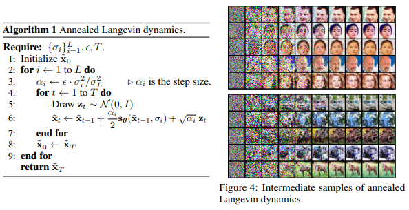
위 방법대로 학습한 모델에서 annealed Langevin dynamics를 이용해 sample을 생성해내는 generative model이다. 순수 Gaussian noise로 부터, step size $\alpha_{1}$으로 $q_{\sigma_{1}}$ 분포에서 T-step Langevin dynamics을 거쳐 sample을 얻는다. 그리고 조금 작아진 step size $\alpha_{2}$로 $q_{\sigma_{2}}$ 분포에서 이전에 얻읃 sample에서부터 시작해 T-step Langevin dynamics을 거쳐 조금 더 원래 data 분포에 가까운 sample을 얻는다. \(\widetilde{x}_{t}=\widetilde{x}_{t-1}+\frac{\alpha_{i}}{2}s_{\theta}(\widetilde{x}_{t-1},\sigma_{i})+\sqrt{\alpha_{i}}z_{t}\;where\;z_{t}\sim N(0,I)\) (\(\nabla_{x}log\,p(\widetilde{x}_{T-1})=s_{\theta}(\widetilde{x}_{t-1},\sigma_{i})\), model의 score를 네트워크로 학습하는 걸 잊지 말자.) 이렇게 쭉쭉쭉 진행해서 noise level이 매우 작아 원래 data 분포에 밀접한 \(q_{\sigma_{L}}\) 분포에서 까지 sampling을 진행한다. 이 때 step size는 noise level의 square에 비례하는 걸 채택했는데, Langevin dynamics에서 SNR ratio가 noise level에 비례하지 않도록 하기 위해서라고 한다. 정확히는 이해 못 함
잠시 DDPM으로 다시 돌아가보자. DDPM도 마찬가지로 순수 Gaussian noise로부터 Langevin Dynamics를 거쳐 원래 data 분포에 가까운 sample을 얻는 점에서 매우 유사하다. 애초에 DDPM 자체가 NCSN을 DPM과 합쳐서 개선한 모델이니, 개선점이 당연히 있겠다. DDPM의 Appendix C에 이런 차이점을 자세히 설명해주고 있다. 우선 NSCN에서는 input의 scaling을 고려하지 않았으나 DDPM에서는 $\sqrt{1-\beta_{t}}$ factor를 forward시에 scale down 해주어서 variance를 1로 고정하는 짓을 했었다. 또한, DDPM sampler와 다르게 NCSN sampler는 post-hoc(SNR ratio가 noise level에 무관하도록 step size를 지정한) coefficients를 사용하기에 sampler가 최적화 되어있음을 보장하지 못한다. 결과를 보고 step size를 저렇게 선택한 건 편법이다!라는 얘기이기도 하고, NCSN 논문에서도 애초에 “Empirically”나 “approximately” 라는게 요 부분에서 자주 보이기도 한다. 그에 비해 DDPM은 forward로 부터 나온 coefficient들을 이용하기에 T step 이후에 분포가 실제 데이터 분포에 일치하도록 sampler가 최적화 되어있다(고 주장했다).
만약 DDPM을 먼저 읽고 NCSN을 처음 접한다면, 딱 여기까지 읽고 DDPM 논문을 다시 읽어보면 예전에는 안 보였던 것들이 보이게 된다.
4. NCSNv2
같은 저자가 같은 모델인 NCSN에 대해서 개선점을 더했는데, 짧게 알아보고 넘어가자.
◼ Noise Scale: 위에서 언급하지는 않았는데, 기존 NCSN에서의 experiment setting은 $\sigma_{1}=1, \sigma_{10}=0.01$로 한 geometric sequence로 구성하였다. 여기서 저자는 1. $\sigma_{1}=1$는 적절한가? 2. geometric sequence는 적절한가? 3. $L=10$은 적절한가?에 대해 모두 다루면서 다음과 같이 얘기했다.
Technique 1 (Initial noise scale). Choose $\sigma_{1}$ to be as large as the maximum Euclidean distance between all pairs of training data points.
Technique 2 (Other noise scales). Choose noise level as a geometric progression with common ratio $\gamma$, such that $\Phi (\sqrt{2D}(\gamma-1)+3\gamma)-\Phi (\sqrt{2D}(\gamma-1)-3\gamma)\approx0.5$ ($\Phi$:CDF of standard Gaussian)
Technique 3 (Noise conditioning). Parameterize the NCSN with $s_{\theta}(x,\sigma)=s_{\theta}(x)/\sigma$, where $s_{\theta}(x)$ is an unconditional score network.
Ideally, we should choose as many noise scales as possible. However, having too many noise scales will make sampling very costly. On the other hand, L=10 as in the original setting is arguably too small.
◼ Annealed Langevin Dynamics: 기존 NCSN에서의 experiment setting은 step size의 coefficient $\epsilon=2\times10^{-5}, T=100$ 이었다. 마찬가지로 이 선택에 대한 이유가 없었기에, 다음과 같은 대답을 내놓았다.
Technique 4(selecting T and $\epsilon$). Choose T as large as allowed by a computing budget and then select an $\epsilon$ that makes equation maximally close to 1. (Equation: $\left (1-\frac{\epsilon}{\sigma_{L}^{2}}\right )^{2T}\left ( \gamma^{2}-\frac{2\epsilon}{\sigma_{L}^{2}-\sigma_{L}^{2}(1-\frac{\epsilon}{\sigma_{L}^{2}})^{2}}\right )+ \frac{2\epsilon}{\sigma_{L}^{2}-\sigma_{L}^{2}(1-\frac{\epsilon}{\sigma_{L}^{2}})^{2}} \approx 1$)
◼ Sampling Stability: 기존 NCSN에서 sampling 중간중간에 갑자기 sample이 튄다던지(색깔이 달라진다던가) 해서 FID score가 튀는 것을 확인했다고 한다. 이는 기존 sampling시 바로 이전의 sample 결과로부터 출발해서인데, 이는 exponential moving average로 쉽게 고칠 수 있다. 즉, 바로 이전의 sample 결과 뿐만 아니라 예전 것들도 적은 가중치로 참고는 하는 것.
Technique 5(EMA). Apply exponential moving average to parameters when sampling.
Reference
Websites
[사이트 출처 1] (https://www.youtube.com/watch?v=KzrdkZUrbPk)
Papers
[1] Hyvärinen, A., & Dayan, P. (2005). Estimation of non-normalized statistical models by score matching. Journal of Machine Learning Research, 6(4).
[2] Vincent, P. (2011). A connection between score matching and denoising autoencoders. Neural computation, 23(7), 1661-1674.
[3] Song, Y., & Ermon, S. (2019). Generative modeling by estimating gradients of the data distribution. Advances in neural information processing systems, 32.
[4] Song, Y., & Ermon, S. (2020). Improved techniques for training score-based generative models. Advances in neural information processing systems, 33, 12438-12448.
[5] Welling, M., & Teh, Y. W. (2011). Bayesian learning via stochastic gradient Langevin dynamics. In Proceedings of the 28th international conference on machine learning (ICML-11) (pp. 681-688).
[6] Du, Y., & Mordatch, I. (2019). Implicit generation and modeling with energy based models. Advances in Neural Information Processing Systems, 32.
[7] Song, Y., Garg, S., Shi, J., & Ermon, S. (2020, August). Sliced score matching: A scalable approach to density and score estimation. In Uncertainty in Artificial Intelligence (pp. 574-584). PMLR.
댓글남기기