[Review] Diffusion Models

Diffusion Model의 기본이라 불리우는 4~5개의 논문에 대한 강의를 보고 정리해보자.

1. Denoising diffusion probabilistic models (DDPM), NeurIPS 2020 ^[2]
2. Denoising diffusion implicit models (DDIM), ICLR 2021 ^[7]
3. Diffusion Models Beat GANs on Image Synthesis (Guided Diffusion), NeurIPS 2021 ^[1]
4. Tackling the Generative Learning Trilemma with Denoising Diffusion GANs (DDGAN), ICLR 2022 Spotlight ^[8]
5. High-Resolution Image Synthesis with Latent Diffusion Models (Stable Diffusion), CVPR 2022 ^[4]

1. Introduction

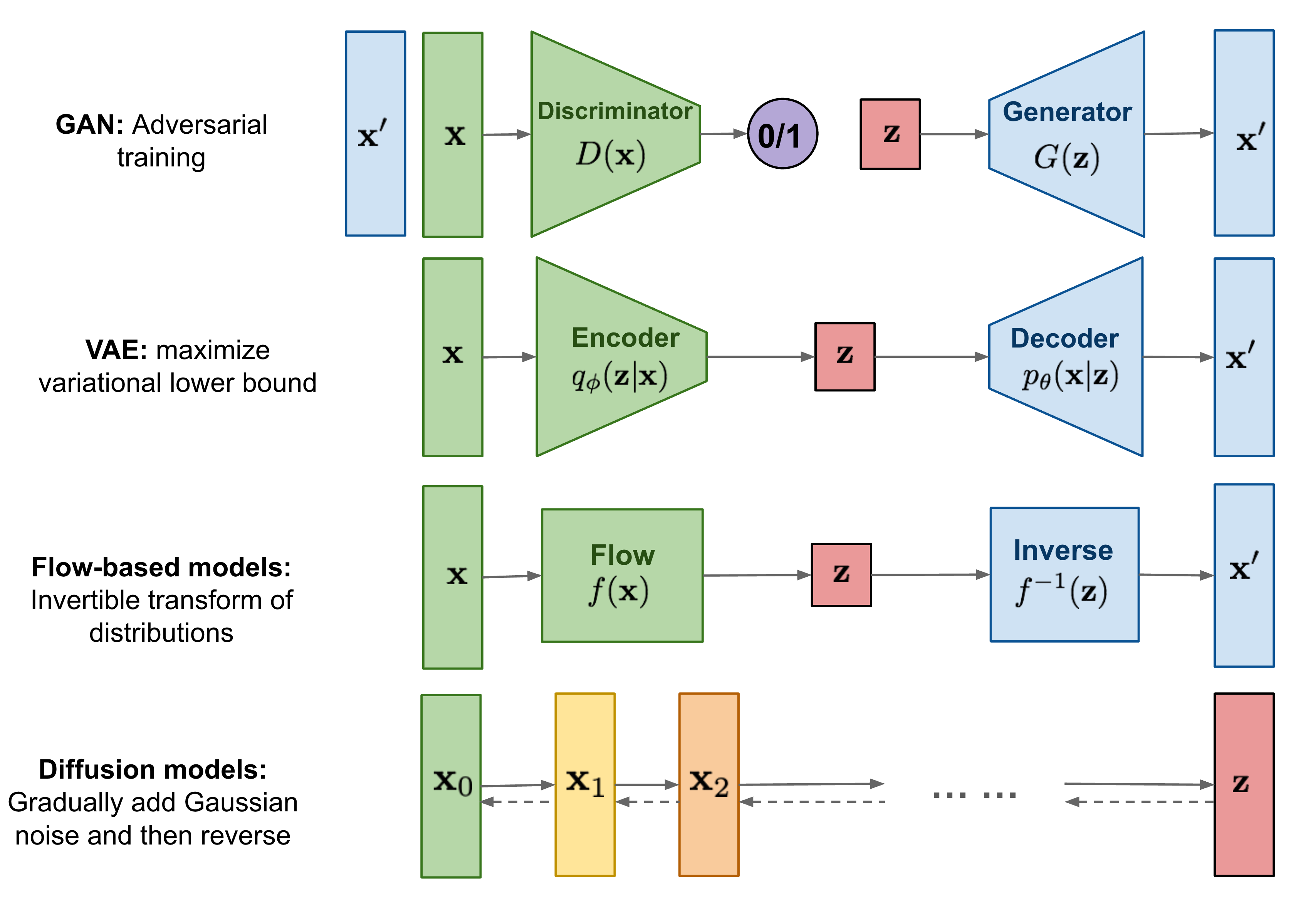
VAE vs. GAN vs. Diffusion

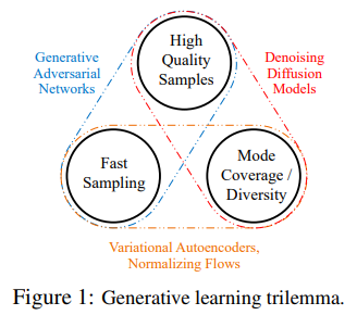
4번 논문에서 각각의 장단점에 대해 잘 설명해둔, 위 두 번째 그림이 있다. GAN은 high quality sample과 빠른 sampling에 장점이 있지만, 다양한 샘플, training distribution을 잘 따라가지 못한다. VAE는 다양한 sample과 빠른 sampling에 장점이 있지만, blur한 sample이 나온다. Diffusion model은 high quality도 되고, 다양한 sample들도 잘 만들지만, sampling이 느리다. 그래서 논문 제목처럼 일종의 trilemma가 있다는 것 같다. 제목 참 잘 지었네…

2. DPM

사실 Diffusion model의 원조는 2015년 발표된 “Deep Unsupervised Learning using Nonequilibrium Thermodynamics”라는 논문이라고 한다. 초창기에는 diffusion process를 통해 Gaussian distribution 같은 well-known distribution으로 부터 target data distribution으로 변환하는 일종의 markov chain을 학습시켜 distribution을 구하고자 하는 모델이다.

Discrete Markov Chain의 property는 잘 알려져있다 싶이, 시간 t+1에서의 확률은 오직 현재 t에만 의존하는 성질이 있다. 즉, Random process가 memoryless property (Markov property라고 했었던 거 같기도 하고)를 가진다.

아무튼 Diffusion model은 기본적으로 data에 임의의 noise를 더해준 후(forward/diffusion process), noise를 제거하는 과정(reverse/denoising process)을 학습하는 모델이다. GAN은 noise로부터 한번에 이미지를 만들지만, Diffusion은 noise를 넣고 빼는 과정으로부터 이미지를 복원하는 거라 살짝 다르다. 여기서 forward process는 $q(X_{t}\mid X_{t-1})$ 확률 (이전 step에서 다음 step의 분포를 구하는 것)을 구하는 과정인데, 이는 정해져있는 것이고 관건은 reverse process. $q(X_{t-1}\mid X_{t})$ 확률 (현재 step에서 이전 step의 분포를 구하는 것)을 구하는 과정인데, 최종적으로 diffusion model의 목표는 이 분포를 학습을 통해 가능하게 만들고자 하는 것이다.

네트워크도 간단한데, time step을 embedding으로 (FC layer를 거친 후) U-net structure network에 넣어줘서 image를 통과시키면 된다.

Forward Process

\(q(X_{t}\mid X_{t-1})=N(X_{t}:\sqrt{1-\beta _{t}}X_{t-1}, \beta _{t}I)\)

즉, $x_{t}=\sqrt{1-\beta_{t}}x_{t-1}+\sqrt{\beta_{t}}\varepsilon$으로 variance를 1로 맞춰주면서 딥러닝 학습이 가능하도록 작은 노이즈를 더해주는, reparameterization trick을 이용한다. input도 normalizaion을 통해 variance가 1이 되도록 맞춰줘야 된다. (안 맞추고 하면 어떻게 될지 궁금하긴 하다) 이 때, $\beta_{t}$는 학습을 할 수도 있겠지만 미리 정해진 상수로 정의해서 forward process에는 학습이 전혀 필요하지 않게 된다. (논문에서는 학습을 해봤는데 상수로 둔 거랑 별 차이가 없었다고 말했다) 또한 $\beta_{t}$의 scheduling을 1e-4~0.02로 점차 증가시키는데 (linear, sigmoid, cosine 등 여러가지 scheduling이 또 가능하겠다.^[3] linear는 너무 빠르게 noise로 변하는 문제가 있어서 cosine 등의 scheduling을 도입했다고 한다.), 처음에는 noise를 조금씩 더하다가 점차 많이 더해가는 느낌이다.

한 방에 적으면,

\[q(X_{t}\mid X_{0})=N(X_{t}:\sqrt{\overline{\alpha_{t}}}X_{0},(1-\overline{\alpha_{t}})I)\;where\;\alpha_{t}=1-\beta_{t},\overline{\alpha_{t}}=\prod_{i=1}^{t}\alpha_{i}\]

즉, 학습할 건 없고 한 방에 계산이 가능하다는 거다.

Reverse Process

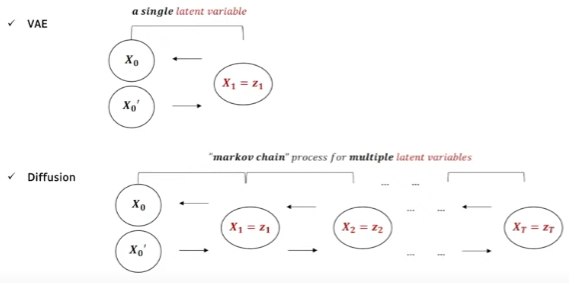
위 그림처럼 VAE는 1개의 latent vector로부터 원래 것을 복원하는 것이라면, diffusion model은 여러개의 step을 통해 만들어낸 여러개의 latent variable들로 부터 markov chain process를 통해 원래 것을 복원하는 것이다. 앞서 말했던 우리의 목표, $q(X_{t-1}\mid X_{t})$ 확률을 알기 위해 이와 유사한 $p_{\theta}(X_{t-1}\mid X_{t})$를 파라미터를 통해 학습하게 된다.

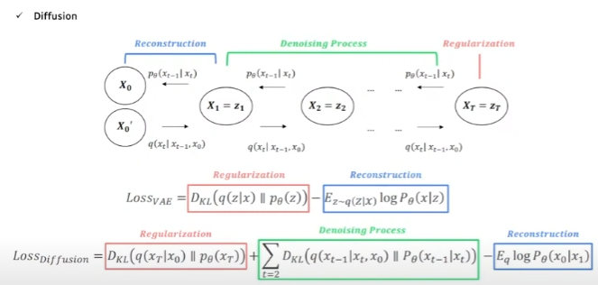
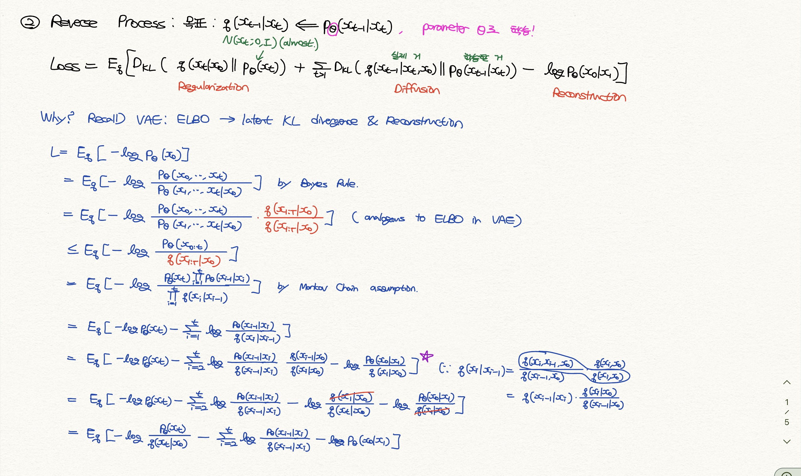
VAE의 loss를 recall해보면 그 복잡한 ELBO하면서 식 전개 해서 나온 loss 함수는 encoder에 KL-divergence로 regularization을 하는 term 하나와, decoder로부터 L1 혹은 L2로 reconstruction loss를 하는 term 이렇게 구성되어 있다.

Diffusion도 비슷하게 식 전개를 한다고 한다. Appendix에 자세히 있는데, 수식이 많아서 다 입력하기 귀찮아 사진으로 대체. 아무튼 KL-divergence로 regularization을 하는 term 하나와, reconstruction loss를 하는 term 두 개가 마찬가지로 포함되어 있다. 여기에 추가로 latent가 여러개라 각 step마다 KL-divergence로 regularization을 하는 term을 더한 항, denoising process term이 추가된다. 식만 보자면 우리가 denoising 하는 $p_{\theta}(X_{t-1}\mid X_{t})$ 분포와, $q(X_{t-1}\mid X_{t})$ 실제 이 분포가 닮도록 해주는 것이다.

DDPM

DDPM^[2]의 공헌은 이 loss term에서 시작된다. 우선 첫 번째 Regularization term을 고려하지 않는다. (상수 취급하는 것과 똑같은 말이다) DDPM 논문의 Section 3.1에서는 이렇게 언급하고 있다.

We ignore the fact that the forward process variances βt are learnable by reparameterization and instead fix them to constants (see Section 4 for details). Thus, in our implementation, the approximate posterior q has no learnable parameters, so LT is a constant during training and can be ignored.

느낌상으로는 $p_{\theta}(X_{t})$는 충분한 forward process를 거쳤기에 $q(X_{t}\mid X_{0})$ 와 같은 Guassian distribution을 이미 잘 따른다고 가정해도 충분하다 뭐 이런 얘기인데, Section 4를 읽어보면 [-1, 1]의 범위로 scaled 된 data에서 $\beta _{t}$를 1e-4~0.02범위로 설정하면 reverse process와 forward process가 거의 같은 functional form을 가져서 이 loss term이 1e-5 bits per dimension, 매우 작아진다고 한다. 그래서 무시하는 건가보다.

그리고 맨 마지막 reconstruction term을 고려하지 않는다. “The variational bound is a lossless codelength of discrete data”라고 section 3.3에 언급되어 있는데, 그냥 저 term이 처음 $\beta _{0}$와 비슷한데 매우 작아서 무시하는 거라고 생각된다. 잘 이해를 못하겠고 여기서도 마찬가지로 input scale [-1, 1]이 역할을 하는게 아닌가 싶다.

DDPM에서 특히 section 4.3 progressive coding와 관련하여 codelength, NLL Test의 bits/dim 뭐 이런 얘기들 하는 부분이 아예 무슨소린지 모르겠어서 그냥 넘어갔다.

3. DDPM

Training

그렇다면 2번째 term이 loss가 될 텐데, 이를 수식적으로 정리할 수 있다. 크게 어려운 건 없고 그냥 Bayes Rule 이용해서 수식 쭉 정리한건데, 쉽지만은 않다. 아래 그림에 수식을 쭉 풀어 놓았다.

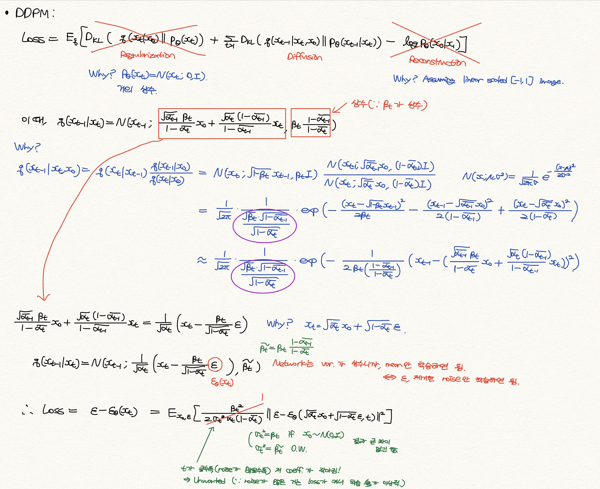
그래서 네트워크는 저 분포에서 variance가 $\tilde{\beta_{t}}$ 로 상수이기에 mean만 학습하면 되고, 그 mean 중에서도 $\beta_{t}$ 나 $\alpha_{t}$ 모두 상수이기에 결국 $\varepsilon$ 만, 즉 제거한 noise만 학습하면 된다.

최종적으로 Loss term은 결국 가우시안 분포를 따르는 $\varepsilon$ 과, 네트워크를 통과한 $\varepsilon_{\theta}(x_{t})$ 과의 L2 loss가 되겠다. 물론 여기서 DDPM에서는 앞에 붙는 coefficient를 1로 고정했는데, 이는 논문 section 3.4에 다음과 같이 언급되어 있다.

In particular, our diffusion process setup causes the simplified objective to down-weight loss terms corresponding to small t. These terms train the network to denoise data with very small amounts of noise, so it is beneficial to down-weight them so that the network can focus on more difficult denoising tasks at larger t terms.

사진에도 있지만, t가 클수록 저 상수가 작아져서 loss가 작아지는데, 사실 noise가 많은 step에서 학습이 많이 되어야 되기에 적합하지 않다고 판단해서 그냥 1로 두었고 그렇다면 noise가 많은 step에서 학습이 많이 되니까 성능이 잘 나온 것 같다. 이 unweighted version에서 $t>1$ case는 NCSN denoising score matching model과 analogous한데, 자세한 건 NCSN를 다룬 내 리뷰에서. [NCSN] DDPM 저자는 Appendix에서 NCSN에서 몇 가지 개선점이 있다고 말하고 있다.

Summary

요 부분만 기억하면 될 것 같다. 구현하는 데 있어서도 이것만 보면 될 듯.

• Forward: \(x_t=\sqrt{\overline{\alpha_{t}}}x_{0}+\sqrt{1-\overline{\alpha_{t}}}\varepsilon \\ \varepsilon\sim N(0,I) \\ \beta_{t}:10^{-4}\searrow 0.02 \\ \alpha_{t}:=1-\beta_{t},\overline{\alpha_{t}}:=\prod_{i=1}^{t}\alpha_{i}\)

• Loss: \(\left \| \varepsilon - \varepsilon_{\theta}(x_{t}) \right \|\)

• Sampling: \(x_{t-1}=\frac{1}{\sqrt{\alpha_{t}}}(x_{t}-\frac{\beta_{t}}{\sqrt{1-\overline{\alpha_{t}}}}\varepsilon_{\theta}(x_{t}))+\sqrt{\tilde{\beta_{t}}}\varepsilon \\ \approx \frac{1}{\sqrt{\alpha_{t}}}(x_{t}-\frac{\beta_{t}}{\sqrt{1-\overline{\alpha_{t}}}}\varepsilon_{\theta}(x_{t}))+\sqrt{\beta_{t}}\varepsilon \\ \tilde{\beta_{t}}:=\beta_{t}\frac{1-\overline{\alpha_{t-1}}}{1-\overline{\alpha_{t}}}\)

4. DDIM

저 위 Summary에서, inference를 할 때 만약에 timestep을 1000번 한다? 그러면 $x_{1000}$ 에서 $x_{0}$를 구할 때 저 sampling process를 총 1000번 하게 된다. 그러면 Forward는 네트워크를 통과하지 않은 단순 계산이라 매우 빠른데, training도 무난한데 추론 시에 연산량이 급격히 많아져서 결과적으로 오래걸리게 된다. “Inference를 할 때 너무 느리니까 조금 더 빠르게 할 순 없을까?” 에 대한 해답을 내놓은 논문이 DDIM.^[7]

Key Idea는 Markov-Chain를 뿌순거다. Non-markov chain을 가정(즉, $x_{t}$가 $x_{t-1}$ 뿐만 아니라 $x_{0}$ 에도 의존)하여 noise를 넣고 빼는데, 우선 forward process를 보면 수학적 귀납법 처럼 증명하여 기존의 DDPM forward 처럼 $x_t=\sqrt{\overline{\alpha_{t}}}x_{0}+\sqrt{1-\overline{\alpha_{t}}}\varepsilon$로 계산할 수 있음을 보였다. (Appendix B Lemma 1) 그리고 Loss term 또한 NonMarkovian 이지만 기존의 loss term과 상수 차이임을 보였기 때문에, 학습에 전혀 지장 없이 기존의 DDPM처럼 $\left | \varepsilon - \varepsilon_{\theta}(x_{t}) \right |$를 활용할 수 있음을 보였다. (Theorem 1)

관건은 Section 4에 나온 Sampling이다. 출처 1에 있는 세미나에서는, “DDPM에서의 paramerization trick, mean에다가 variation 더해서 하는 게 아니라 DDIM에서는 deterministic하게 정하는 것에 차이가 있다. 즉, $x_{t-1}= \sqrt{\overline{\alpha_{t-1}}}x_{0}+\sqrt{1-\overline{\alpha_{t-1}}}\varepsilon_{t-1}=\sqrt{\overline{\alpha_{t-1}}}x_{0}+\sqrt{1-\overline{\alpha_{t-1}}-\sigma_{t}^2}\varepsilon_{t}+\sigma_{t}\varepsilon$ 요 식에서 Markov Chain이 아니기 때문에 $\varepsilon_{t-1}$ term이 붙는데, 이를 또 DDPM에서 했던 방식대로라면 저렇게 mean에다가 $\sigma_{t}\varepsilon$를 더해주는 식으로 하는데, 그게 아니라 $\sigma_{t}$를 0으로 해서 deterministic 하게 하였다.” 라고 말하고 있다. 요 얘기가 정확히 Section 4.1에서 나오고 있으며, $\sigma_{t}$를 0으로 했을 때 resulting model이 implicit probabilistic model이 되어서 (Diffusion은 아니지만) 이를 DDIM이라고 부르자 라고 되어 있다. 이게 Section 4.3에서 “DDPM은 $dt$에 대해서, DDIM은 $d\sigma$에 대해서 inference를 한다. sampling step을 줄였을 때, $\alpha_{t}$와 $\alpha_{t-\Delta t}$가 충분히 가깝지 않아 DDPM과 차이가 난다.” 뭐 이렇게 얘기하고 있는데, 무슨 소린지 모르겠다. 정확한 이해를 위해서는 SDE 논문을 좀 읽어봐야 될 것 같다. 곧 SDE의 시초인 논문 3편을 읽어볼 예정.

Summary

여하튼 sampling만 조금 다르게 해서 더 빠르게 할 수 있겠다.

• Forward: \(x_t=\sqrt{\overline{\alpha_{t}}}x_{0}+\sqrt{1-\overline{\alpha_{t}}}\varepsilon \\ \varepsilon\sim N(0,I) \\ \beta_{t}:10^{-4}\searrow 0.02 \\ \alpha_{t}:=1-\beta_{t},\overline{\alpha_{t}}:=\prod_{i=1}^{t}\alpha_{i}\)

• Loss: \(\left \| \varepsilon - \varepsilon_{\theta}(x_{t}) \right \|\)

• Sampling: \(x_{t-1}=\sqrt{\overline{\alpha_{t-1}}}(\frac{x_{t}-\sqrt{1-\overline{\alpha_{t}}}\varepsilon_{\theta}(x_{t})}{\sqrt{\overline{\alpha_{t}}}})+\sqrt{1-\overline{\alpha_{t-1}}}\varepsilon_{\theta}(x_{t})\)

Implementation

Pytorch_Diffusion

Phil Wang 씨의 pytorch implementation이 잘 되어 있어서 이걸 사용하고 있다. 코드 업데이트가 이루어질까봐 우선 내 레포로 복사해두었다. 몇 가지 디테일 한 사항으로는

1. DDPM 작가는 Wide ResNet block을 썼으나, 해당 코드에서는 그냥 typical conv. layer을 써서 groupnorm과 함께 사용하였다. 원래는 WeightStandardizedConv2d를 구현해두었으나 삭제된 것으로 보인다. Kolesnikov et al., 2019
2. Linear attention variant도 구현되어 있다. 입맛에 따라 사용 가능. Shen et al., 2018
3. U-net에는 (batch_size, in_channels, height, width)와 (batch_size, 1)이 들어가서 (batch_size, in_channels, height, width)가 나온다. 처음에 noisy image는 conv layer를 거치고 noise level는 position embedding layer를 거쳐 time embedding을 계산한다. 그리고 downsampling (ResNetx2 + RMSNorm + Attention + Residual + downsample), middle stage (ResNet + Attention + Residual + ResNet), upsampling (ResNetx2 + RMSNorm + Attention + Residual + upsample), 이후 마지막 ResNet+conv를 거친다.
4. 위에서 잠깐 얘기했었던, $\beta_{t}$의 scheduling도 여러 개 구현되어 있다. Nichol et al., 2021^[3]
5. GaussianDiffusion class에서 objective parameter로 ‘pred_noise’, ‘pred_x0’, ‘pred_v’ Salimans and Ho, 2021를 선택할 수 있다. typical 하게는 pred_noise를 고를 수 있겠다.
6. auto_normalize parameter는 True로 설정 시, torchvision.transforms Compose에서 ToTensor() 시의 범위 [0, 1] 범위를 자동으로 [-1, 1] 범위로 만들어 준다.
7. q_sample이 forward process이고, sample이 reverse inference이다. (이는 @autocast 되어 있는 것과, @torch.inference_mode() 되어 있는 것으로 확인할 수 있다.) sampling_timesteps parameter를 timesteps parameter보다 작게 주었을 때 자동으로 ddim_sampling이 되며 (ddim_sampling_eta로 eta 값 조절 가능), 그렇지 않을 경우 p_sample_loop가 된다.

이처럼 간단하게 소개해둔 huggingface의 좋은 사이트가 있다. The Annotated Diffusion Model 그리고 원래 구현해주신 분의 레포에 denoising-diffusion-pytorch guided_diffusion (#5), classifier_free_guidance (#7) 등등 다른 것들도 구현되어 있으니 나중에 참고하면 좋을 것 같다.

5. Guided Diffusion^[1]

논문 이름도 참 잘 지었다. 특히 Abstract 첫 문장, “We show that diffusion models can achieve image sample quality superior to current SOTA models.” 이걸 보고 안 읽을 사람이 어디있겠냐…

이 논문의 기여는 크게 두 가지로, 1. Unconditional image synthesis는 Architecture 수정. 2. Conditional image synthesis는 Classifier Guidance 라는 걸 도입. 해서 성능을 올렸다.

Architecture Improvements

Section 3에 나와 있는 것 처럼, 크게 5가지 정도를 변경하였다.

1. 전체 model size는 비슷하되, depth versus width를 증가시켰다.
2. Multi-head attention. Attention head를 증가시켰다.
3. Multi-resolution attention. 16x16만 있는 것이 아닌, 32x32, 16x16, 8x8 resolution attention을 사용하였다.
4. SDE 논문에서 처럼, activations upsampling/downsampling에 BigGAN residual block을 이용하였다.
5. Residual connection rescaling factor를 $1/\sqrt{2}$로 하였다.

추가적으로는 Adaptive Group Normalization을 하였는데, 이는 StyleGAN에 나왔던 adaptive instance norm과 비슷하게 $y_{s}GN(h)+y_{b}$식으로 한다.

Classifier Guidance

DDPM, DDIM에서는 단순히 분포 $p_{\theta}(x_{t} \mid x_{t+1})$를 학습했다면, label이 주어진 conditional image synthesis에서는 t 시점에서 이미지가 무엇인지, 그 label까지 반펼하는 것을 고려한다. 즉, 분포 $p_{\theta, \phi}(x_{t} \mid x_{t+1},y)$ 를 학습한다. $p_{\theta, \phi}(x_{t} \mid x_{t+1},y)=Zp_{\theta}(x_{t} \mid x_{t+1})p_{\phi}(y \mid x_{t})$ 에서 $p_{\theta}(x_{t} \mid x_{t+1})$는 정규분포 $N(\mu, \Sigma)$를 따르고, $p_{\phi}(y \mid x_{t})$는 log 취해서 근사 때려가지고 $log(p_{\theta}(x_{t} \mid x_{t+1})p_{\phi}(y \mid x_{t}))\approx -\frac{1}{2}(x_{t}-\mu-\Sigma g)^{T}\Sigma ^{-1}(x_{t}-\mu-\Sigma g)+C$로 나타낼 수 있다. 이 때, g는 $\nabla_{x_{t}}logp_{\phi}(y \mid x_{t})\mid_{x_{t}=\mu}$로 classifier 분포 log 취해서 taylor 근사 때릴때 튀어나오는 친구이다.

그래서 DDPM에서 했던 것 처럼 $\mu, \Sigma$에서 $x_{t-1}$을 sampling 하는게 아니라, $N(\mu+s\Sigma\nabla_{x_{t}}logp_{\phi}(y \mid x_{t}), \Sigma)$에서 sampling하는 것이다. 여기서 s는 scaling factor로 Section 4.3에 소개되어 있는데, 요약하자면 s를 증가시킬수록 model의 diversity는 감소하지만 fidelity(이미지 quality)는 증가하는 trade-off가 있다.

DDIM과 비교하자면, Sampling시 활용했던 $\varepsilon_{\theta}(x_{t})$ 대신 $\hat{\varepsilon}=\varepsilon_{\theta}(x_{t})-\sqrt{1-\overline{\alpha_{t}}}\nabla_{x_{t}}logp_{\phi}(y \mid x_{t})$를 활용하여 sampling을 한다.

끝으로 저자가 unlabeled data에도 clustering을 통한 synthetic label을 통해 classifier guidance technique을 활용할 수 있도록 해보겠다~고 말하고 있다.

6. DDGAN^[8]

말 그대로 DDPM + GAN. Diffusion model이 GAN보다 느린 대신 fidelity가 높기 때문에 두 가지 장점(만)을 모두 가져보자 하는 것 같다.

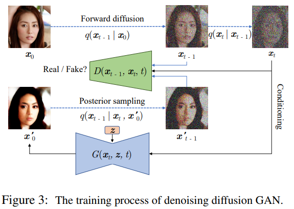
원본 이미지 $x_{0}$에서 forward process를 통해 $x_{t-1}$과 $x_{t}$를 계산하고, $x_{t}$를 Generator에 넣어서 $x_{0}’$을 만든다. 기존 DDPM, DDIM은 $x_{t}$에서 여러 step을 거쳐 $x_{0}’$을 추론한다면, 요 모델에서는 그냥 Generator에 통과시켜서 한 방에 $x_{0}’$을 만든다. 그러고 나서 주어진 $x_{t}, x_{0}’$를 통해 Reverse process로 $x_{t-1}’$을 만든다면, Discriminator는 $x_{t-1}, x_{t-1}’$을 넣어주어서 Real인지 Fake인지 구분하도록 한다. 정말 말 그대로 Diffusion model에 GAN을 활용한 구조.

7. Stable Diffusion^[4]

Latent Diffusion 이라고도 불리는, 핫 한 모델. Diffusion model에서 reverse inference는 DDIM을 통해서 sampling step을 줄였기에 속도를 올릴 수 있었지만, 여전히 충분하지 못한 step은 fidelity에 문제가 있기 때문에 결국 여전히 느린 문제가 있다.

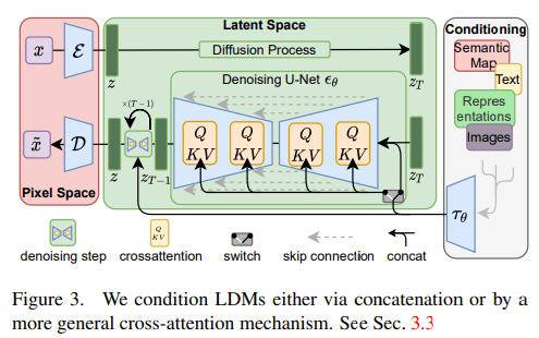
그래서 이 모델에서 이를 개선하고자, image data의 pixel space (3x256x256)에서 diffusion을 거치는 것이 아니라, 위 그림처럼 pre-trained encoder를 거쳐서 latent space (cxhxw)에서 diffusion을 거친 후 decoder를 거치는 과정을 하게 되었다.

해당 논문의 실험에서 FFHQ dataset을 제외하고는 CelebA-HQ dataset 등등에서는 이를 1/4배 (또는 1/8배) 하여 256x256이 아닌 64x64의 data가 diffusion에 들어가게 된다. 대략적으로 생각해도 computational cost가 약 16배 줄어드는 셈. 결국 남은 문제는 성능이 잘 나오느냐인데, text-to-image synthesis로 유명한 느낌이 없지 않아 있지만 text 뿐만이 아닌 layout(semantic map) 등등의 conditional image synthesis, super-resoluion task (고해상도 이미지로 변환하는 task), inpainting task(이미지 일부가 소실되었을 때 복원하는 task) 등에서도 성능이 매우매우 좋다고 말하고 있다.

Text-to-image

Section 4.3에 나와 있는 정보에 의하면, BERT-tokenizer를 이용해 CLIP text encoder (transformer architecture)를 LAION dataset에서 training을 한다. 그리고 autoencoder는 ImageNet 기반으로 1/4배, 1/8배로 줄이는 모델을 학습하였다. 이게 latent-space에서 1/8배 시에는 KL-regularization을 하는데 1/4배 시에는 또 아니고 뭐 이런 detail이 있는 것 같은데 일단 스킵. 그리고 이런 pre-trained parameter를 가지고 본격적으로 diffusion에 활용되는 U-Net을 학습하게 된다. Github에 제공된 것은 LAION 5B dataset을 통해 학습하였다고 되어 있는데, 이게 용량이 거의 85TB던데 ㄷㄷ

이 때, U-Net에서 self-attention이 아니라 cross-attention mechanism을 활용하여 conditioning 기능을 하도록 하였다. 기존의 self-attention이라면 input(지금 같은 경우에는 image의 feature map)에서 Query Q, Key K, Value V를 모두 뽑아와서 $Attention(Q,K,V)=softmax(\frac{QK^{T}}{\sqrt{d_{k}}})V$를 계산한다. 그러나 여기서 활용하는 Cross attention은, image의 feature map 뿐만 아니라 pre-trained CLIP text encoder를 거친 text embedding도 있어서 요 두가지를 모두 활용하는 메커니즘이다. 즉, image의 feature map에서 Query Q를 뽑고, text embedding에서 Key K, Value V를 뽑아서 계산하는 것이다.

이렇게 했을 때의 장점으로는, 1. text embedding의 Value V 값에서 특정 V를 크게 함을 통해서 특정 단어를 강조하는 역할을 할 수 있다. 2. image feature의 Query Q, text embedding의 Key K 값, $QK^{T}$에서 masking을 적용하면 특정 단어를 무시하는 역할을 할 수 있다. “Prompt-to-Prompt Image Editing with Cross Attention Control”이라는 논문에서 이러한 fine-tuning 방식이 자세히 설명되어 있는데, 예를 들어 “Children drawing of a castle next to a frozen river”라는 문장이 있다면, 1. frozen에 해당하는 token의 value 값을 증가시키면 좀 더 강이 얼어붙은 모습이 나오는 그림이 나오고, Children drawing에 해당하는 value를 증가시키면 아이가 그린 듯한 그림이 나오는 것 2. 의미가 없는 전치사나 상대적으로 의미가 적은 next to 같은 단어는 무시할 수 있는 것이다. 물론 이런 것들은 fine-tuning training 하면서 알아서 학습하는 거고 이를 해석하는 것 뿐이다.

또한, 위 Guided Diffusion에서 소개한 Classifier guidance가 아닌, 학습된 classifier가 필요 없는 Classifier free guidance를 사용했다. Classifier-free diffusion guidance 논문을 자세히 보지는 않았지만, $\varepsilon_{\theta}(x_{t})-s\nabla_{x_{t}}logp_{\phi}(y \mid x_{t})$가 아닌 $\varepsilon_{\theta}(x_{t},c)-\varepsilon_{\theta}(x_{t},\phi)$를 이용하는데. c는 text embedding, $\phi$는 빈 text embedding이다. scaling factor도 text 길이 등에 대한 느낌으로, Classifier guidance와 유사하게 s가 클수록 텍스트를 많이 반영하는 느낌으로 fidelity가 증가함과 동시에 diversity는 감소한다. 이렇게 해서 classifier를 사용하지 않고 puer한 diffusion model이 classifier guidance에서 얻은 유사한 trade-off를 가지면서 높은 fidelity의 sample을 얻게 된다. 생각해보면 단순히 Bayes Rule, $\nabla_{x_{t}}logp_{\phi}(y \mid x_{t})=\nabla_{x_{t}}logp_{\phi}(x_{t} \mid y)-\nabla_{x_{t}}logp_{\phi}(x_{t})$ 를 적용한 것이라 그리 어려운 건 아니다. Classifier free guidance 논문 저자는 기존의 Classifier guidance가 noise level 마다 classifier를 학습해야 하는 단점이 있고, classifier에 기반해 모델을 평가하는 IS/FID score를 편법처럼 올린 것이라고 주장해 좌변이 아닌, 우변과 같은 항을 채택했다. 그래서 학습 시에는 $\nabla_{x_{t}}logp_{\phi}(x_{t} \mid y)$는 $\varepsilon_{\theta}(x_{t},c)$에 해당하고, $\nabla_{x_{t}}logp_{\phi}(x_{t})$는 class label을 drop out한 상태인 $\varepsilon_{\theta}(x_{t},\phi)$를 이용하는 것이다. Sampling 시에는 둘 다 써서 classifier guidance와 동일한 효과를 결국 얻게 되는 것. 아무튼.

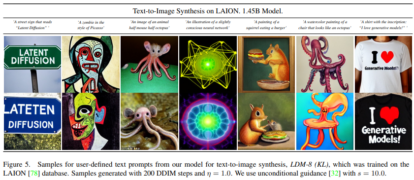
KL-regularized x1/8 latent space로 보내는 LDM 모델에서, DDPM ($\eta=1.0$이라) sampling 200 steps 및 classifier free guidance with s=10.0을 사용하였고 그 결과이다.

8. DreamBooth^[5]

Stable diffusion의 fine-tuning 방식으로는 Textual Inversion, DreamBooth 등 여러 논문들이 있지만 또 구글이 낸 논문은 읽어봐야 될 것 같아서 DreamBooth를 간략히 정리해보았다.

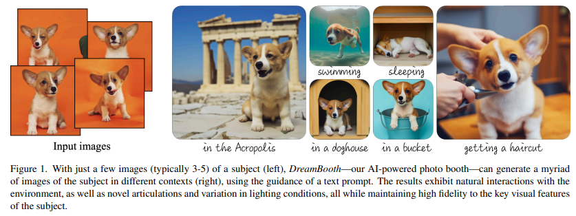
Few shot (3~5장 정도)으로 fine-tuning을 해서 위 그림처럼 dog 이미지 몇 장을 주면 수영하고 있는, 해외에서 자고 있는 dog를 만들 수 있다. 물론 이렇게 tuning한 모델을 cat에 적용하려면 또 다시 모델을 fine-tuning 해야 되고, V100 기준 30분 정도 걸린다고 한다.

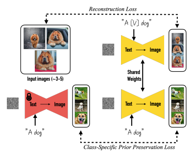
큰 틀은 2개의 loss로 구성되어 있다. 첫 번째 reconstruction loss는, fine-tuning할 stable diffusion model에 text-embedding으로 “A [V] dog”를 넣은 결과와 input간 L2 loss이다. 이 때 [V]는, 논문에서는 T5-XXL tokenizer의 rare-word를 사용했고 “xxy5syt00”처럼 random character를 이으면 hazardous way라고 하는데, 실제 다른 분들 구현한 것을 보면 “sks”처럼 아무 의미없는 랜덤 단어를 넣어도 잘 돌아가는 것 같다. 두 번째 Class-specific prior preservation loss는, 기존의 갖고 있던 stable diffusion model의 파라미터를 freeze한 채로 text input을 “A dog”를 주었을 때 나온 결과와, fine-tuning할 stable diffusion model에 text-embedding으로 “A dog”를 넣은 결과와 input간 L2 loss이다. 이 prior-presevarion loss가 있을 경우 dog의 자세나 얼굴 모습이 동일하게 나온다는 등 다양성에서 문제가 조금 있다고 말하고 있다.

Reference

Websites

[사이트 출처 1] https://www.youtube.com/watch?v=jaPPALsUZo8

[사이트 출처 2] https://www.youtube.com/watch?v=Z8WWriIh1PU

[사이트 출처 3] https://huggingface.co/blog/annotated-diffusion

[사이트 출처 4] https://github.com/lucidrains/denoising-diffusion-pytorch/tree/main

Papers

[1] Dhariwal, P., & Nichol, A. (2021). Diffusion models beat gans on image synthesis. Advances in Neural Information Processing Systems, 34, 8780-8794.

[2] Ho, J., Jain, A., & Abbeel, P. (2020). Denoising diffusion probabilistic models. Advances in Neural Information Processing Systems, 33, 6840-6851.

[3] Nichol, A. Q., & Dhariwal, P. (2021, July). Improved denoising diffusion probabilistic models. In International Conference on Machine Learning (pp. 8162-8171). PMLR.

[4] Rombach, R., Blattmann, A., Lorenz, D., Esser, P., & Ommer, B. (2022). High-resolution image synthesis with latent diffusion models. In Proceedings of the IEEE/CVF Conference on Computer Vision and Pattern Recognition (pp. 10684-10695).

[5] Ruiz, N., Li, Y., Jampani, V., Pritch, Y., Rubinstein, M., & Aberman, K. (2023). Dreambooth: Fine tuning text-to-image diffusion models for subject-driven generation. In Proceedings of the IEEE/CVF Conference on Computer Vision and Pattern Recognition (pp. 22500-22510).

[6] Salimans, T., & Ho, J. (2022). Progressive distillation for fast sampling of diffusion models. arXiv preprint arXiv:2202.00512.

[7] Song, J., Meng, C., & Ermon, S. (2020). Denoising diffusion implicit models. arXiv preprint arXiv:2010.02502.

[8] Xiao, Z., Kreis, K., & Vahdat, A. (2021). Tackling the generative learning trilemma with denoising diffusion GANs. arXiv preprint arXiv:2112.07804.

[9] Ho, J., & Salimans, T. (2022). Classifier-free diffusion guidance. arXiv preprint arXiv:2207.12598.